PNR Models and Fitting Basics

PNR Models

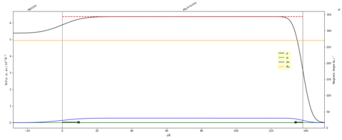
When fitting PNR data, the objective is to find a physically reasonable model that well-represents the structural and magnetic depth profiles of the thin film or multilayer being probed. In order to do this, Refl1D represents the sample as a series of slabs with fittable parameters such as thickness, interface roughness, or nuclear and magnetic scattering length density. In the simplest cases, each layer of the film may be represented as a single layer with constant SLDs as shown in the example below.

In contrast to this basic case, it is true the case that features exist in the depth profile which are not account for so simply. Magnetically dead layers may develop, drift may occurs during film depositions, or interfacial intermixing may give rise to an alloyed layer at the interface. In all of these examples, it may be necessary to represent a layer which was intended to be nominally uniform as more than one slab layer in Refl1D. It is also possible for the physics of a thin film structure to require more complex shapes, and in these advanced cases Refl1D supports features such as functional forms for SLD profiles or the fitting of the depth profile through a series of control points connected by spline functions. Thus, a sample with a magnetization which varies exponentially throughout the depth, so that M(Z) = A×e^B×Z may be readily represented, with both A and B as fittable parameters. 

We provide examples of these more advanced cases in the example library.

Algorithms and χ² Optimization

The Refl1D software program fits data by using a variety of algorithms for optimization of reduced χ², possessing a particularly powerful suite of fitting engines. Due to the large number of variables generally used to fit a PNR dataset, one must be particularly careful in determining whether a fit optimizer has in fact arrived at the globally best (lower χ²) solution, or merely become stuck in a local minima. Although this page is intended to provide an extremely basic practical  introduction to PNR fitting, we do recommend interested readers consult the complete documentation for more difficult fitting problems. That being said, there are three fitting engines most commonly employed at the NCNR:

• Nelder-Meade Simplex: Fast, but slightly more likely to get stuck in a local minimum. Use for cases in which many parameters are already well know or tightly constrained, and for relatively simple structures. Doing multiple restarts of the algorithm can mitigate the tendency to get stuck. Probably the best at getting to the very lowest χ² if the starting point is good.
• Differential Evolution: Medium speed, much more likely to find the global minimum
• DREAM: Slowest, with very high memory requirements for export and processing. Good for more fully exploring the parameter space and estimating uncertainty. This is a population-based Monte-Carlo algorithm with multiple different start points which can be initialized in a variety of different ways. Selecting "lhs" (latin hypersquares) spreads the start points out relatively evenly to better cover the parameter space, while "eps" starts everything near the initial guess and is better for uncertainty analysis.