PBR Experiment

PROPAGATION OF EXCHANGE BIAS COUPLING ACROSS A REGION UNDERGOING A FERROMAGNETIC PHASE TRANSITION  

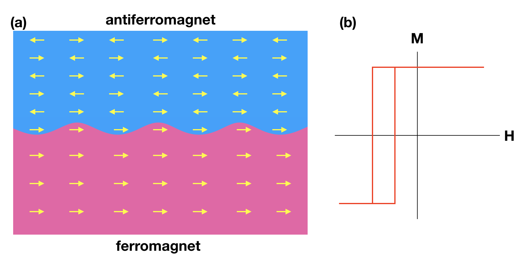
Exchange bias is a special type of magnetic anisotropy that can manifest in a ferromagnet when interfaced with an antiferromagnet [1].  An (over)simplified depiction of this phenomenon is shown in Figure 1(a).  In general, there is no net magnetization associated with an antiferromagnet, as neighboring spins align antiparallel, canceling each other out.  However, if an antiferromagnet is cooled through it’s ordering point (Neel temperature, T_N), in the presence of a modest external magnetic field, symmetry breaking near an imperfect interface can lead to a relatively small number of spins that are uncompensated and aligned in the same direction.  Because these interfacial spins are still very strongly coupled to the antiferromagnetically ordered bulk, they are pinned, meaning an extremely large magnetic field is required to rotate them.  Below the ferromagnetic transition (Curie temperature, T_C) ordered spins in the ferromagnet can then couple to the interfacial pinned spins in the antiferromagnet, leading to a preferred magnetization direction for the ferromagnet, as shown in Fig. 1(b).  This is known as unidirectional magnetic anisotropy or exchange bias, and is exploited for a multitude of applications in magnetic recording and sensor technology.  

Despite the widespread utilization of exchange bias, basic questions of the underlying mechanisms are still being explored, including efforts to understand the role of magnetic order in the bulk of the antiferromagnet [2] and the ferromagnet [3], as opposed to just at the interfaces. Here, we consider the case of an exchange biased ferromagnet with T_C that varies with distance away from the antiferromagnet / ferromagnet interface.  Specifically, we will examine an exchange biased T_C “well” where the ordering temperature is lower in the middle of the layer than it is at the top or bottom [4].  At high temperature (below T_C of the top and bottom ferromagnetic regions, but above that of the center region), the top and bottom magnetizations will be placed in an decoupled, antiparallel configuration, and we will examine how the magnetic depth profile evolves as the low T_C center undergoes a ferromagnetic phase transition.  The thin film multilayer sample was grown via magnetron sputtering by Kristen Repa from Casey Miller’s group at the Rochester Institute of Technology, and is depicted in Figure 2. 

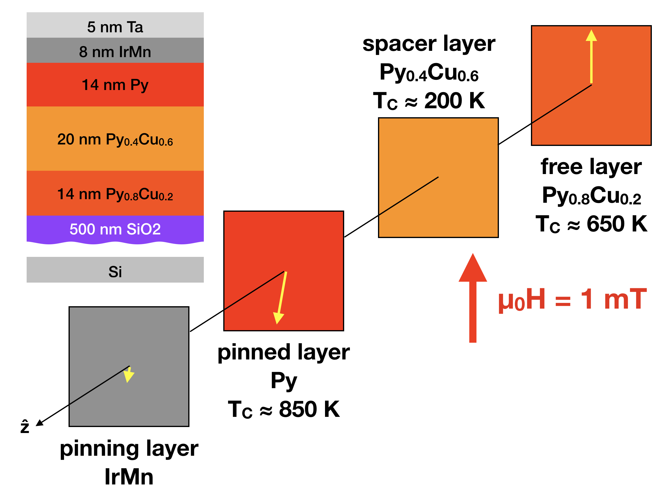
The biasing antiferromagnet is IrMn, while the ferromagnetic material is Py_xCu_1-x,  an alloy of permalloy, Ni₈₀Fe₂₀ (abbreviated Py) with non-magnetic Cu to control T_C.  The layer closest to the antiferromagnet is the pinned layer, and is comprised of pure Py, with a nominal T_C \(\approx\) 850 K.  We refer to the subsequent Py_0.4Cu_0.6layer as the spacer layer, which has a much lower T_C \(\approx\) 200 K.  Below that is the Py_0.8Cu_0.2 free layer, with T_C \(\approx\) 650 K.  At room temperature (293 K) we can safely assume that the outer pinned and free layers are ferromagnetic, while the center spacer layer is not.  In this case, there is no means of direct exchange between the pinned and free layers, making those layers essentially uncoupled to one another[5]. Therefore, we should be able to place the pinned and free layers into a stable antiparallel state by applying a weak magnetic field antiparallel to the biasing direction of the IrMn, as shown in Fig. 2.   What we aim to find out is what happens as the sample is cooled below the T_C of the Py_0.4Cu_0.6 spacer.  As ferromagnetic order takes hold in that layer, it finds itself in a complex energy landscape, with coupling to the pinned Py layer promoting magnetization in one direction, and coupling to the free Py_0.8Cu_0.2 layer promoting magnetization in exactly the opposite direction.  Will the bias from the antiferromagnet propagate through the entire stack?  Which way will the spacer magnetization spontaneously orient?  Will the layer magnetize uniformly, or break up into domains?  Will the layer mediate coupling between the other layers?  If so at what temperature? 

To investigate this phase transition, we will use the PBR beamline to perform specular polarized neutron reflectometry (PNR), a technique sensitive to the depth profiles of the nuclear composition and magnetization [6]. Using a narrowly collimated, monochromatic (wavelength 0.475 nm) neutron beam, we will measure measure the spin-dependent reflectivities as a function of wavevector transfer along the sample growth direction (Q_z) using a ³He pencil detector.  The sample will be mounted inside a closed-cycle refrigerator, and an electromagnet will be used to apply a magnetic field H perpendicular to both the sample growth direction and the neutron propagation direction (i.e. field applied vertically).  An Fe/Si supermirror / Al-coil spin flipper assembly will be used to polarize the incident neutron magnetic moment either parallel (+) or antiparallel (-) to H. A second supermirror/flipper array will be used to analyze the spin state of the scattered beam.

The Q_z-dependent reflectivity is determined by the depth dependence of the scattering length density, which has both nuclear and magnetic components.  The nuclear scattering length density is defined

$$\rho_{N} = \sum_{i} N_{i}b_{i},\tag{Eq. 1}$$

where N is the number density, b is the nuclear scattering length corresponding to a particular isotope [7], and the summation is over each isotope present in the scattering volume, and provides information about the chemical composition of the sample.  For our purposes here, the magnetic scattering length density is defined as a vector quantity, 

$$\overrightarrow{\rho_{M}} = C\overrightarrow{M} ,\tag{Eq. 2}$$

where \(\overrightarrow{M}\) is the sample magnetization (magnetic moment per unit volume) and the constant C  = 2.91 x 10-9 for \(\rho_{M}\) in units of Å^-2 and M in units of kA m^-1 (or emu cm^-3).  The non spin-flip reflectivities R⁺⁺ and R^{- -} tell us about \(\rho_{N}\) and the in-plane component of \(\rho_{M}\) parallel to H.  Within the Born Approximation

$$ R^{\pm \pm}(Q_{z}) = \frac{16 \pi^{2}}{Q_{z}^{2}} \left |\int_{-\infty}^{+\infty}e^{iQ_{z}z} \left[ \rho_{N}(z) \pm \rho_{M}(z) \cos \phi_{M}(z)\right]dz\right |^{2} \tag{Eq. 3 } $$

where \(\phi_{M}\) is the angle between \(\overrightarrow{M}\) and \(\overrightarrow{H}\).

The spin-flip scattering tells us about the in-plane magnetization perpendicular to H.  We can usually [8] assume that R^-+and R^+- are the same, such that again, within the Born Approximation, 

$$ R^{+-}(Q_{z}) = R^{-+}(Q_{z}) = \frac{16 \pi^{2}}{Q_{z}^{2}} \left |\int_{-\infty}^{+\infty}e^{iQ_{z}z} \left[ \rho_{M}(z) \sin \phi_{M}(z)\right]dz\right |^{2} \tag{Eq. 4 } $$

Thus, measurement of all four polarization states allows us to determine the structural and in-plane vector magnetization depth profiles.  While the Born Approximation is useful for providing a simple qualitative picture of the relationship between reflectivity and scattering length density, it fails catastrophically near total external reflection.  Fortunately, it is straightforward to use the optical transfer method to exactly calculate the reflectivity corresponding to any any arbitrary sld profile [6].  As such, we can determine the depth profiles via model fitting of the reflectivity data.  We will do this using the Refl1D software package [9].  

The reflectivity measured for our sample in a 500 mT saturating field parallel to the bias direction at 40 K is shown in the top panel of  Figure 3, while the profile determined from the fit to this data is shown in the bottom panel.  

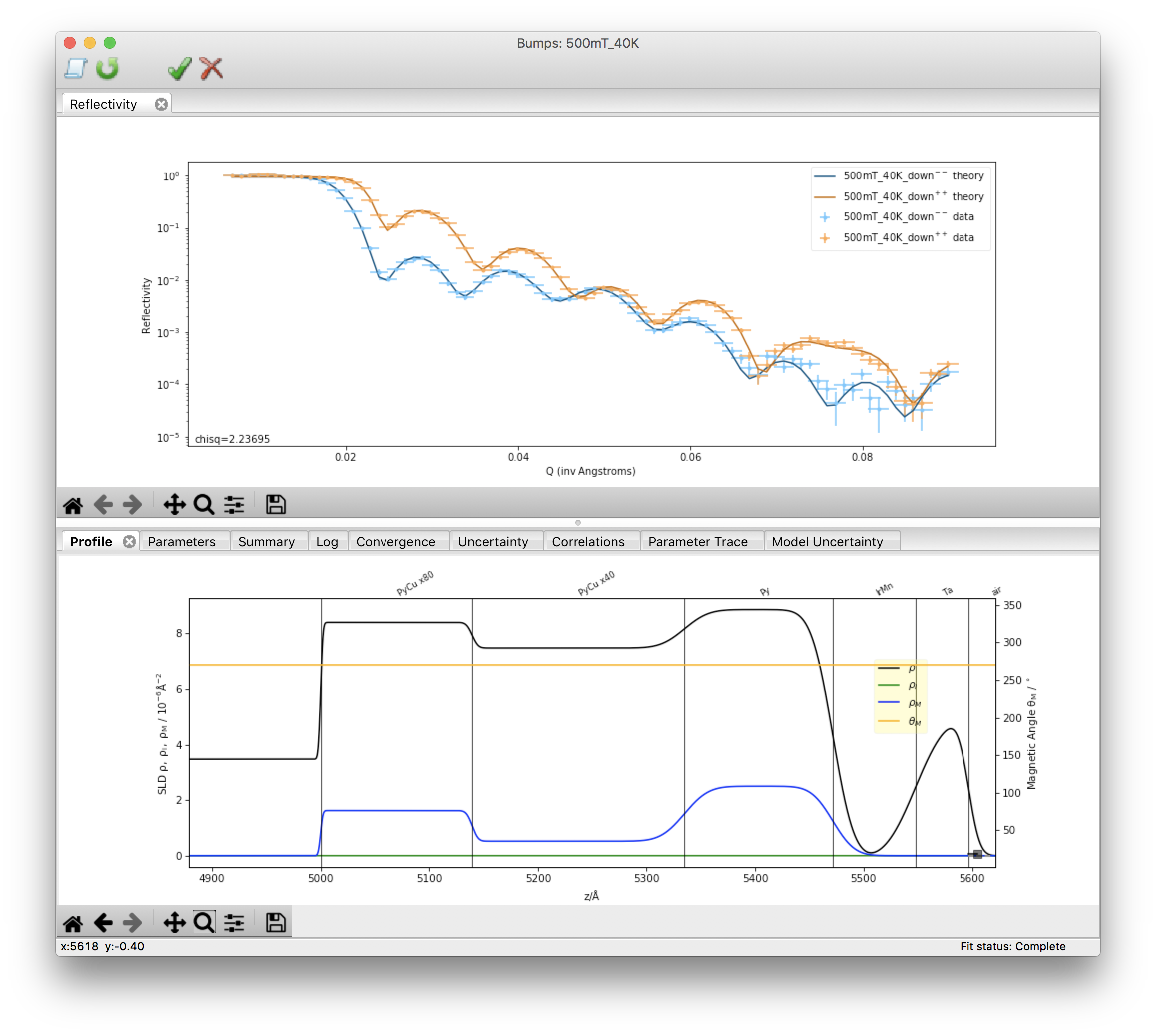
We see features in \(\rho_{N}\) corresponding to each of the expected layers, and non-zero \(\rho_{M}\) for the three ferromagnetic layers.  This is because all competing fields (i.e. the biasing and applied magnetic fields ) are oriented in the same direction (and the applied magnetic field is strong enough to align the magnetizations of all the ferromagnetic layers anyway). For the bulk of the antiferromagnetic IrMn \(\rho_{M}\) should be zero, as the ordered spins should perfectly cancel, and (while certainly good enough to see the contributions from the ferromagnet) the statistical quality and Q_z-range of the data are insufficient for us to reasonably distinguish any weak \(\rho_{M}\) corresponding to the pinned interfacial magnetization [10].  Thus the data are modeled well with a IrMn layer featuring zero \(\rho_{M}\).  We will use this model as the basis for modeling our temperature-dependent data.

For our experiment, we will start with the sample at 300 K, and will apply a 700 mT saturating field (enough to align the magnetization of all layers except for the pinned spins of the IrMn) antiparallel to the IrMn bias direction (marked on the sample).  The field will then be reduced to a near remanent 1 mT.  This should result in an antiparallel alignment of the pinned and free layers, similar to what is shown in Fig. 2.  We will then take PNR measurements as a function of decreasing temperature in order to examine the evolution of the magnetic depth profile as ferromagnetism emerges in the Py_0.4Cu_0.6 spacer layer.  

[1] J Nogués, and Ivan K Schuller. Journal of Magnetism and Magnetic Materials , 192, 203 (1999). 
[2] R. Morales, Zhi-Pan Li, J. Olamit, Kai Liu, J. M. Alameda, and Ivan K. Schuller, Physical Review Letters 102, 097201 (2009)
[3] R. Morales, Ali C. Basaran, J. E. Villegas, D. Navas, N. Soriano, B. Mora, C. Redondo, X. Batlle, and Ivan K. Schuller. Physical Review Letters 114, 097202 (2015).
[4] A. F. Kravets, A. N. Timoshevskii, B. Z. Yanchitsky, M. A. Bergmann, J. Buhler, S. Andersson, and V. Korenivski. Physical Review B 86, 214413 (2012).
[5] Here we are concerned with direct exchange between layers, which should provide the dominant contribution to any interlayer coupling for this system.  However there are means of indirect exchange (e.g. RKKY coupling) which can play significant roles in metallic magnetic multilayers.
[6] C. F. Majkrzak, K.V. O’Donovan, and N.F. Berk. “Polarized Neutron Reflectometry.” In Neutron Scattering from Magnetic Materials, 397–471. Elsevier, 2006.
[7] https://ncnr.nist.gov/instruments/magik/Periodic.html
[8] There are special (and interesting!) situations where this would not be the case for this scattering geometry (e.g. helical magnetism). 
[9] http://refl1d.readthedocs.io/en/latest/
[10]  However, while challenging, you can distinguish those pinned spins with PNR!   see M. R. Fitzsimmons, M, B. J. Kirby, S. Roy, Zhi-Pan Li, Igor V. Roshchin, S. K. Sinha, and Ivan K. Schuller.  Physical Review B 75, 214412 (2007).