
Official websites use .gov
A .gov website belongs to an official government organization in the United States.
Secure .gov websites use HTTPS
A lock (
) or https:// means you’ve safely connected to the .gov website. Share sensitive information only on official, secure websites.
Searching for Magnetic Skyrmions in Powdered B20 Materials with SANS
Introduction
Magnetic skyrmions are wrapped spin structures in which magnetic moments in a material form a continuous closed planar structure, as shown in Figure 1a [1, 2]. The core and perimeter of the skyrmion point out of the plane of the film in opposite directions. These features together give the skyrmion a topological protection which makes it robust against system defects. In addition to the topological qualities of skyrmions, their small size (typically 20 nm - 300 nm) and relative mobility - achieved with moderate charge currents - makes these structures a promising approach for next-generation, ultra-high density memory and logic technologies.
In typical magnetic materials, all of the magnetic moments align parallel (ferromagnetism) or anti-parallel (antiferromagnetism). The wrapped skyrmion spin structure is distinctly different and arises due completion between the traditional Heisenberg direct-exchange term, which takes the form J(S1·S2), and an exotic anti-symmetric exchange coupling termed the Dzyaloshinskii-Moriya interaction (DMI), which takes the form D(S1×S2). While the dot product in the direct exachge prefers parallel or antiparallel alignment between spins, the cross-product in the DMI interaction introduces an additional energy term which motivates the magnetic moments to orient at 90° relative to each other.
Skyrmions naturally form in some non-centrosymmetric materials, most commonly with the B20 structure, with the most frequently studied materials being MnSi[3], FeGe[4], and Cu2OSeO3[5]. In these materials, in a limited magnetic field and temperature range corresponding to an ideal balance between the direct exchange, DMI, dipole energy, magnetocrystalline energy and thermal energy, skyrmions populate the sample. These skyrmions form in the plane orthogonal to the applied magnetic field and order into hexagonally packed arrays, shown in Figure 1b. The small size and magnetic-only contrast of these structures makes it extremely challenging to directly investigate them. The most common approaches are direct imaging with Lorentz TEM, Figure 1c, and small angle neutron scattering (SANS), Figure 1d.
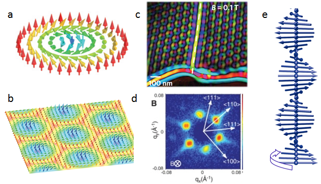
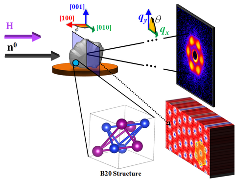
The first experimental observation of magnetic skyrmions was reported in 2009, with the key piece of evidence provided by small angle neutron scattering, shown in Figure 1d [3]. In a typical SANS investigation of skyrmions, the incident neutrons are parallel to the magnetic field (and hence orthogonal to the skyrmion lattice), as illustrated in Figure 2 [6]. In the SANS scattering geometry, the neutrons diffract from any regular lattice structure, giving rise to a reciprocal space diffraction pattern (shown on the right of Figure 2) which is the Fourier transform of the real-space structure. For the case of hexagonally-packed skyrmions, the Fourier transform is simply a hexagon.
In typical skyrmion materials, coupling between the magnetism and the underlying crystalline lattice defines the orientation of the hexagonally-packed skyrmion array. Thus, for a single crystal, if the magnetic field is applied in a plane which has low-symmetry, the skyrmions within the material will order into a well-defined lattice with a common preferential orientation that gives rise to the six distinct peaks in the SANS scattering pattern (Figure 2). If, for example, the sample is prepared in a higher symmetry orientation, the SANS pattern may have 12 or more peaks due to contributions from all the domains in the sample. For this reason, almost every SANS experiment on skyrmions is performed on large single crystals - large to achieve sufficient material for SANS, and single crystal to have long range coordination between the structural and magnetic lattices. Performing a SANS experiment on a powder or polycrystalline material, one would expect the SANS pattern to be the sum of the skyrmion hexagon patterns from every randomly-oriented crystallite, which will appear as a ring. Unfortunately, a ring is not useful for uniquely identifying or characterizing the skyrmion phase since, in a powder, it is also consistent with the formation of simple magnetic helices (Figure 1e) in random directions - or really any structure with a defined periodicity and no net orientation. For these reasons the search for new skyrmion materials using SANS is extremely challenging, and has focused only on single crystals, rather than powders, even though high quality crystals are much harder to produce.
Rotating skyrmions in a magnetic field
The goal of this experiment is to develop a technique to precipitate ordered, oriented skyrmion lattices in disordered powdered samples to rapidly screen candidate materials. The challenge is to distinguish the helical phase from the skyrmion phase even though their scattering signature (i.e., ring) is the same. The proposed approach builds on the observation that the orientation of a hexagonal skyrmion lattice in a single crystal can be rotated by introducing a symmetry-breaking anisotropy using electric field[7], uniaxial pressure [8] or spin-transfer torque [9]. These approaches, however, require that the material have sufficient magnetocrystalline anisotropy to define the original orientation of the skyrmion lattice. It has similarly been demonstrated [6], that the skyrmion state in a single crystal with weak anisotropy can be altered by physically rotating the crystal in a static magnetic field. Since the skyrmion lattice necessarily is stabilized in the plane orthogonal to the magnetic field and the field is not moving, the lattice rotates within the sample in response. As the sample is twisted, the skyrmions traverse through a complex landscape of the crystal's magnetocrystalline energies, intrinsic defect sites which can pin the sample, and also interactions with other skyrmions (which may be caught on a pinning site). It is not immediately clear what the effect of rotation in a field will have on the magnetic order in a disordered powdered sample, but you can probably guess that it is relevant to this experiment.
The Proposed Experiment
In this experiment we will be investigating the effects of rotating a skyrmion-containing powder of Cu2OSeO3 (The onset of magnetic order is TC=58 K, Figure 3) [5] in a static magnetic field. From a fabrication standpoint powders are much easier to fabricate than large single crystals, but the skyrmion lattices are misaligned. Furthermore, powders are particularly challenging in SANS since the large structural disorder gives rise to a strong effective background that we are not particularly interested in. We will rotate the powder sample at T>TC, T=57 K and H=0.2 T (which should be the ferromagnetic state), T=57 K and H=0.3 T, which should be the skyrmion state, and T=45 K and H=0.3 T, which should be the helical state.
![Figure 3 Stability diagram taken from [5] for Cu2OSeO3.](/sites/default/files/styles/480_x_480_limit/public/images/2018/06/06/ng7sans_c_fig3.png?itok=GOgbuQhp)
The SANS Instrument
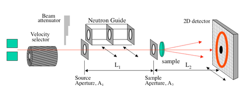
SANS instrument NG7 [10], illustrated in Figure 4, is optimized to cover a q-range of 0.008 nm-1 to 7 nm-1, which translates to features sizes below 1 nm and up to 500 nm. Recall that q (sometimes denoted Q) = 2π sin(α)/λ ≈ 2π/distance, where α is the scattering angle on the detector with respect to the transmitted neutron beam center. The neutron wavelength (λ) may be tuned between 0.5 nm and 2 nm with a wavelength spread between 11% and 22% full-width half-maximum.
The intensity of the scattering on the detector after background correction in the SANS experiment is given by
$$I_{meas} = \phi A dT\left( \frac{d\Sigma}{d\Omega} \right) \Delta \Omega \varepsilon t$$
where
\(\phi\) is the number of neutrons per second per unit area incident on the sample
\(A\) is the sample area
\(d\) is the sample thickness
\(T\) is the sample transmission
\(\Delta \Omega\) is the solid angle over which scattered neutrons are accepted by the analyzer
\(\varepsilon\) is the detector efficiency
\(t\) is the counting time
The aim of the SANS experiment is to obtain the differential macroscopic scattering cross-section dΣ/dΩ from Imeas. Data reduced in this way are said to be on “absolute scale” and should be easily comparable from one neutron scattering facility to another.
Planning the Experiment
Scattering Length Density
In order for there to be small-angle scattering, there must be scattering contrast. In this case the nuclear structure of the crystallites embedded in a matrix of vacuum provides one contrast, while the magnetic structure (periodic chiral structure or saturated state) provides a second. The scattering is proportional to the scattering length density (abbreviated SLD or symbolized as ρ) squared. SLD is defined as
$$ \rho = \frac{1}{V} \sum_i^n b_i $$
where V is the volume containing n atoms, and bi is the (bound coherent) scattering length of the ith atom in V. V is usually the molecular or molar volume for a homogeneous phase in the system of interest.
Neutrons are scattered either through interaction with the nucleus (nuclear scattering, N) or through interaction between the unpaired electrons (and hence the resultant magnetic moment, M) and the neutron spin. Hence, Cu2OSeO3 has both a nuclear SLD and a magnetic SLD and will display both nuclear and magnetic contrast.
Nuclear SLDs can be calculated from the above formula, using a table of the scattering lengths [11] for the elements, or calculated using the interactive SLD Calculator available at the NCNR’s web pages [12]. Magnetic SLD can be calculated using the following formula
$$ \rho_m = M\left( in\, \mathrm{\frac{A}{m}} \right) \times 2.853 \times 10^{-12} \mathrm{\frac{m}{A {\unicode{x212B}}^{-2}}} $$
Some handy magnetic conversions are:
$$ \mathrm{ \frac{A}{M}} = 1000 \mathrm{ \frac{emu}{cm^3} }; \mu_B = 9.274 \times 10^{-21} \mathrm{emu} $$
The magnetic saturation of bulk Cu2OSeO3 is 513 emu/cc. With a density of 5.07 g/cm3 and a saturation magnetization of 24.8 emu/cm3, the nuclear SLD can be calculated to be 5.27 ×10‑6 Å‑2 and magnetic SLD as 7.09 ×10⁻⁸ Å-2. We note that the nuclear scattering is ≈20× larger than the magnetic scattering.
Sample Thickness
Given the calculated sample contrast, how thick should the sample be? Recall that the scattered intensity is proportional to the product of the sample thickness, ds, and the sample transmission, T. It can be shown that the transmission, which is the ratio of the transmitted to the incident beam intensity, is given by
$$T = e^{-\Sigma_t d_s} $$
where \( \Sigma_t = \Sigma_c + \Sigma_i + \Sigma_a \) (the sum of the coherent, incoherent, and absorption macroscopic cross sections). The absorption cross section, \( \Sigma_a \) , can be accurately calculated from tabulated absorption cross sections of the elements (and isotopes) if the mass density and chemical composition of the sample are known. The incoherent cross section, \( \Sigma_i \) ,can be estimated from the cross section tables for the elements as well, but not as accurately as it depends on the atomic motions and is, therefore, temperature dependent. The coherent cross section, \( \Sigma_c \) , can also only be estimated since it depends on the details of both the structure and the correlated motions of the atoms in the sample. This should be no surprise as \( \Sigma_c \) as a function of angle is the quantity we are aiming to measure!
The scattered intensity is proportional to dsT and hence
$$ I_{meas} \propto d_s e^{-\Sigma_t d_s} $$
which has a maximum at \(d_s = 1/\Sigma_t \) and implies an optimal transmission at \( 1/e = 0.37 \). However, one must also be wary of multiple scattering for transmissions less than ≈ 0.90.
SASCALC
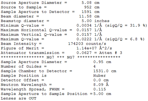
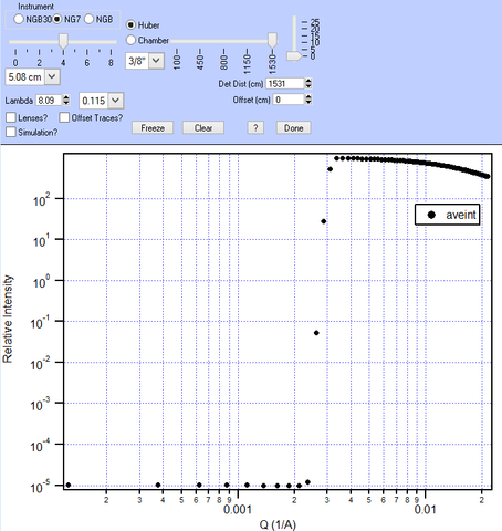
SASCALC is a tool built into the SANS IGOR reduction package that allows different beamline configurations to be simulated, helping users to select an ideal balance between desired q-range and maximum beam intensity. The nominal size of the skyrmions is 70 nm in Cu2OSeO3, which corresponds to a q of 0.09 nm-1 (0.009 Å-1) Based on this, a reasonable configuration for the instrument can be calculated to be:
We may optimize these further and/or run an additional, higher-q configuration.
Magnetic scattering
The measured scattering intensity, I, is proportional to the squared sum of the spatial nuclear (N2) and magnetic (M2) Fourier transforms, defined as
$$ N, M_J(\mathbf{q}) = \sum_K \rho_{N,M_J} (K) e^{i\mathbf{q} \cdot \mathbf{R_K}} $$
where J is any Cartesian coordinate, ρN,M is the nuclear or magnetic scattering length density, and RK is the relative position of the Kth scatterer. Note that because we can only measure the absolute value of the Fourier Transform squared in a scattering experiment, rather than the complex components of the Fourier Transform itself, we lose phase information. The result is that we may not be able to uniquely distinguish between a family of curves that model our data – a fact that should be kept in mind during data fitting and analysis.
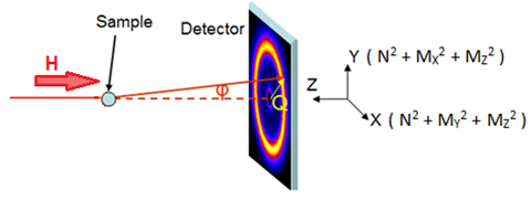
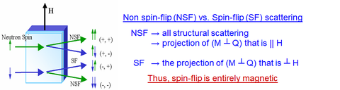
Additionally, in neutron scattering only the component of a magnet moment oriented perpendicular to the scattering wave vector, q, participates in scattering [3]. Thus, for a detector set in the X-Y plane, all three magnetic components can be observed at various angles, see Figure 5. For this experiment, the magnetic field, H, will be aligned along the Z-direction.
The challenge in many experiments is to distinguish the magnetic scattering (M2) from the nuclear scattering (N2) which dominates. Additional information about the magnetic scattering can be gained by polarizing the incident and/or scattered neutron beam and selecting out one of the neutron spin states (spin-up or spin-down). Polarizing devices, such the optional supermirror in the incident beam, allows one spin state to be transmitted while the other spin state is reflected away, resulting in a polarized neutron beam. If a small magnetic field is maintained which varies slowly in direction with respect to the neutron’s Larmor precession frequency, the beam will remain polarized along the entire flight path. The difference between spin-down and spin-up scattering allows one to highlight the scattering from the net magnetic moment || to H (at the point of sample scattering), M||, by recovering a nuclear-magnetic cross-term, NM||. This can be helpful in cases where the magnetic scattering signal is weaker than the structural scattering. Finally, by also analyzing the spin orientation after scattering from the sample, the scattering from all three magnetic components (MX, MY, and MZ) can be obtained – a procedure beyond the scope of this experiment, but a summary of which can be found in the Supplementary Information section.
Data Reduction and Processing
The SANS IGOR Analysis package [13] will be used to properly scale and reduce your data onto an absolute scale. In order to do this, you will need to collect several types of data files. Transmissions are collected with the beam stop removed (translated to the side) in order to survey the unscattered neutron beam; these are taken with a series of attenuating filters to insure this main neutron beam isn’t so intense so as to burn the detector. Scattering files, on the other hand, make use of a beam stop that blocks this main beam in order to emphasize the weaker sample scattering observed at higher angles. In this case, a sufficiently large beam stop (1” to 4” possible depending on detector distance and beam collimation) is chosen so that attenuating filters are typically not required. Note that a transmission file will be used to define the beam center (from which Q is calculated), while a scattering file will be used to align the beam stop with respect to the main beam.
An abbreviated list of the data reduction steps includes:
- Sample scattering files will be acquired at 15 m detector distance to cover an optimal q-range
- Corresponding transmission files of the sample (powder+foil packet), empty (sample holder only), and open beam will be used to determine [and correct for] absorption.
- The “open” transmissions described above will additionally be used for absolute-scale intensity normalization.
- “Empty” scattering files will be taken to remove the scattering resulting from the sample holder + any main beam spillover (around the beam stop)
- Background scattering files will be taken using a beam block in order to remove electronic noise and spurious neutron scattering from nearby experiments
- Radial projections will be performed and are expected to show combined nuclear structure and magnetic structure
- Azimuthal projections will be performed at a q corresponding to the magnetic feature to identify any textured symmetry in the chiral system
Data will be reduced using three approaches. In approach (1) measurements will be corrected for sample holder background contributions to highlight the total nuclear plus magnetic scattering, (2) measurements above TC or in saturation will be subtracted as background, thus removing the structural component of the scattering. , and(3) the difference in scattering of the spin-up and spin-down neutrons will be subtracted, thus highlighting the magnetic component of the SANS pattern that is || H.
Data Analysis/Modeling
SANS data can be analyzed [14] using the IGOR Pro SANS software previously used for data reduction [13] and/or the SasView Package [15]. It is particularly easy to evaluate the 2D SANS symmetry within the IGOR Pro SANS software. However, once your data have been circularly or sector averaged into 1D [Intensity versus Q] plots, both IGOR and SasView have a suite of prebuilt models that can be utilized. An advantage of SasView is that existing models can be quickly combined or custom-made models can be created using C or Python code that can describe almost any imaginable morphology. Designing a custom-built model is beyond the scope of this experiment, but it is worthwhile to keep in mind for future SANS experiments.
Scattering symmetry via IGOR Pro SANS software:
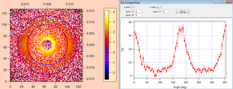
Upon recalling a raw, 2D data set (SANS Reduction Controls → Raw Data → Display Raw Data) or reducing a data set onto absolute scale (SANS Reduction Controls → Reduction → Build Protocol), an azimuthal average can be performed within IGOR using I vs. Q → Average Panel (pink pop-up box) → Annular average. This is depicted below in Figure 6. This treatment allows the symmetry of the system to be quickly evaluated. To save the azimuthal slice in text format, use Average Panel, check Save File to Disk → Do Average. Alternatively, you may wish to save an I vs. Q circular or sector average using I vs. Q → Average Panel (pink pop-up box) → Circular/Sector average, check Save File to Disk → Do Average.
Modeling I vs. Q via SasView:
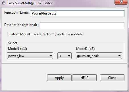
Data can be loaded and viewed using Load Data → select file → Send To [Fitting]. An example of a skyrmion circular average minus at high temperature background is shown as blue circular data points in Figure 7. Under Model, you will see there are many Shape-Independent, Shapes, and Structure Factor models to choose from. However, in this example case, the data requires both a low-q Power Law slope to describe the nuclear scattering plus a Gaussian peak model to describe the magnetic skyrmion scattering.
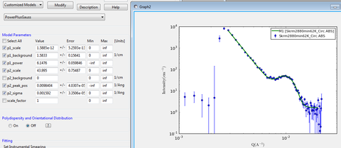
Models may be easily combined starting from the tab Fitting → Edit Custom Model → Sum, as depicted in Figure 8. This new model, named PowerPlusGauss, will show up under Model → Category → Customized Models. Once selected, it will appear on the same graph alongside the data (see green curve of Figure 6). It is recommended that the available parameters are adjusted by hand until the model comes close to representing the data set. After that, specific parameters of interest may be selected (checked boxes in Figure 6) and optimized using the Fit function in SasView. Note, there are many fitting algorithms to choose from under Fitting → Fit Options. Additionally, the q-range considered, polydispersity of the parameters, and whether to include instrumental smearing are available options to consider. We will go over the fitting procedure in more detail during the summer school.
References
[1] Fert, et al., Nat. Nanotechnol. 8, 152 (2013).
[2] Nagaosa et al., Nature Nano. 8, 899 (2013)
[3] A. Mühlbauer et al., Science 323, 915 (2009)
[4] FeGe Citation
[5] S. Seki et al., Science 336, 198 (2012)
[6] D. A. Gilbert et al., Under Review
[7] White J. S., et al. Electric field control of the skyrmion lattice in Cu 2 OSeO 3. J. Phys.: Condens. Matter 24, 432201 (2012).
[8] Chacon A., et al. Uniaxial Pressure Dependence of Magnetic Order in MnSi. Phys. Rev. Lett. 115, 267202 (2015).
[9] Everschor K., et al. Rotating skyrmion lattices by spin torques and field or temperature gradients. Physical Review B 86, 054432 (2012).
[10] Glinka et al., J Appl. Cryst. 31, 430 (1998)
[11] V.F. Sears, Neutron News 3, 29-37 (1992)
[12] https://www.ncnr.nist.gov/resources/activation/
[13] S. R. Kline, J. Appl. Cryst. 39, 895 (2006); http://www.ncnr.nist.gov/programs/sans/data/red_anal.html
[14] ftp://ftp.ncnr.nist.gov/pub/sans/kline/Download/SANS_Model_Docs_v4.10.pdf
[15] http://www.sasview.org/
Supplementary Information On Spin Selection Rules
The original rule (discussed for unpolarized neutrons in section 4d) that only the component of M ┴ Q can participate in scattering also holds true for polarized neutrons. Additionally, of this projection of M ┴ Q, the part that is also || to the neutron polarization axis (defined by H) does not reverse the neutron spin. The remaining projection of M ┴ Q that is ┴ to the neutron polarization axis (defined by H) does reverse the neutron spin. These processes are denoted as non spin-flip (NSF) and spin-flip (SF) scattering, respectively. The nuclear scattering does not affect the neutron spin, and so all structural scattering is confined to the NSF scattering. These rules are summarized in Figure 9.
While it is beyond the scope of this experiment, please note that polarization analysis allows for the measurement of magnetic scattering even if it is (a) dominated by the structural scattering or (b) not aligned with an applied magnetic field, but randomly oriented in space such that its net sum is zero. The applied magnetic field required to align the neutron spins may be quite small (say 0.005 Tesla or less).