
Official websites use .gov
A .gov website belongs to an official government organization in the United States.
Secure .gov websites use HTTPS
A lock (
) or https:// means you’ve safely connected to the .gov website. Share sensitive information only on official, secure websites.
AMB2022-01 Benchmark Measurements and Challenge Problems
Modelers are invited to submit simulation results for any number of challenges they like before the deadline of 23:59 (ET) on July 15, 2022. Tabulated results using the challenge-specific templates are required. A Q&A webinar will be held on May 5, 2022 for the metals benchmarks (01 – 05) and on May 6, 2022 for the polymers benchmarks (06 – 08). Registration has closed. After the webinar is completed, links to the recorded presentations and to a FAQ page will be added to this description page. For convenience, a .pdf of this entire “AMB2022-01 Benchmark Measurements and Challenge Problems” description document can be found in the content below. Additional information may become available later so updated versions of this document may be posted. Please check back occasionally.
All evaluations of submitted modeling results will be conducted by the AM-Bench 2022 organizing committee. Award plaques will be awarded at the discretion of the organizing committee. Because some participants may not be able to share proprietary details of the modeling approaches used, we are not requiring such details. However, whenever possible we strongly encourage participants to include with their submissions a .pdf document describing the modeling approaches, physical parameters, and assumptions used for the submitted simulations.
Please note that the challenge problems reflect only a small part of the validation measurement data provided by AM Bench for each set of benchmarks. The Measurement Description section, below, describes the full range of measurements conducted.
AMB2022-01: Laser powder bed fusion (LPBF) 3D builds of nickel-based superalloy IN718 test objects. Detailed descriptions are found below. Submissions have closed.
Challenges
- Time Above Melting Temperature (CHAL-AMB2022-01-TAM): Time above the midpoint between the solidus and liquidus temperatures for the melt pool at specified locations within the build volume. This metric is closely related to melt pool length but is explicitly location specific.
- Solid Cooling Rate (CHAL-AMB2022-01-SCR): Cooling rate immediately following complete solidification (below solidus) at specified locations within the build.
- Residual Elastic Strains (CHAL-AMB2022-01-RS): Residual elastic strain components at select locations internal to the bridge structure, corresponding to synchrotron X-ray diffraction measurements.
- Part Deflection (CHAL-AMB2022-01-PD): Deflection of the as-built (no heat treatment) bridge structure after it is partially separated from the build plate.
- Microstructure (CHAL-AMB2022-01-MS): Histograms of direction-specific grain sizes from specified regions within as-built and heat-treated samples.
- Phase Evolution (CHAL-AMB2022-01-PE): Formation and evolution of phases and phase fractions, including major precipitates, as a function of time for heat treatments of IN718 from a 2.5 mm leg.
- Overview and Basic Objectives
- Build and Post-Build Processing Description
- Measurement Descriptions
- Benchmark Challenge Problems
- Data to be Provided
- Relevant References
Jump to: Section 1 | Section 2 | Section 3 | Section 4 | Section 5 | Section 6
1. Overview and Basic Objectives
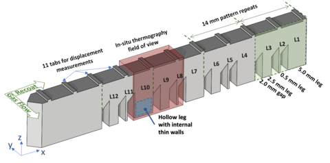
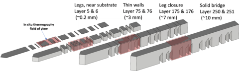
The AMB2022-01 benchmarks use laser powder bed fusion (LPBF) 3D metal alloy builds of a bridge structure geometry that has 12 legs of varying size, as shown in Figure 1. All of the legs are solid except for leg 10 that is hollow with thin internal walls.
The modeling challenges fall into five areas: the local cooling rates immediately before and after solidification, the time above melting temperature, residual strain field within the part while attached to the base plate, distortion of the part after partial cutting from the base plate, and the location-dependent microstructure in as-built and heat-treated conditions. We emphasize that modelers who wish to submit simulation results are free to address any number of challenges. Partial submissions to individual challenges will also be accepted.
All provided data, including precursor material characterization, scan strategy, part CAD files, and example measurement results data can be found using the links in Section 5 and throughout this document.
2. Build and Post-Build Processing Description
2.1 Materials and Part Design
2.1.1 Substrates:
Nickel alloy IN718 AM parts are built on substrates (build plates) consisting of nominally the same alloy. The substrates are 100 mm squares, 12.5 mm thick, and mounted from below using four ¼-20 cap screws in direct contact with a custom 304 stainless steel baseplate. Substrates also included two k-type thermocouples mounted to the underside, described further in Section 2.3.3.
2.1.2 Part layout on the build plate:
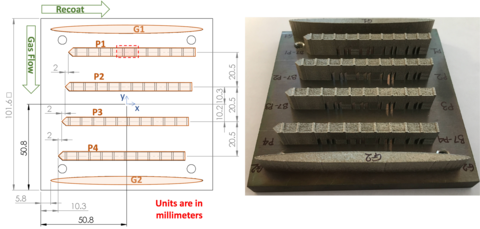
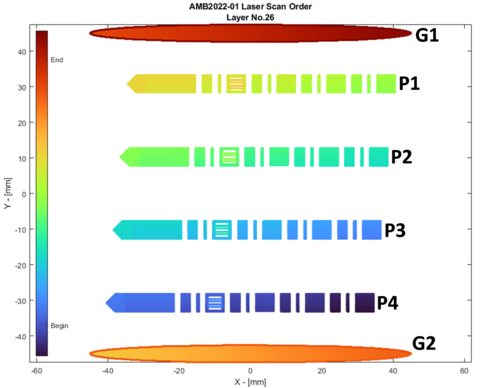
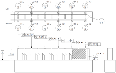
Four bridge-structure parts (labeled P1 to P4) and two recoater guides (labelled G1 and G2) are fabricated on each build plate, as shown in Figure 2. Each bridge part is identical. They are spaced by 20.5 mm along the Y-axis, and they are offset from each other along the X-axis by 2.0 mm so that the recoater blade progressively engages each one. The guides G1 and G2 are solid structures used to ensure the recoater does not damage the bridge structures. The recoating direction and laminar gas flow direction are also shown. Stereolithography (STL) and STEP files which includes CAD geometry of the build plate, parts, and their relative locations can be found in the /CAD_Geometry/ directory of the AMB2022-01 challenge description dataset.
Note that users should refer to the AMMT scan strategy description and data (Section 2.3) for more precise positioning of parts with respect to the AMMT coordinate system. The AMMT coordinate system is based on the laser-scanning positions, therefore references to the edge of the build plate are approximations.
2.1.3 Individual part geometry:
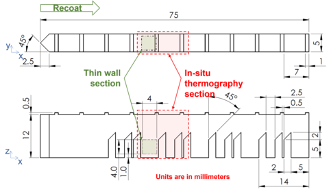
Figure 3 presents a schematic of the bridge structure part that is 75 mm long, 12 mm tall, and 5 mm wide with 7 mm tall ‘legs’ that form into 45° overhangs below a solid structure. The recoating direction starts at the pointed end with the 45° taper, and proceeds left. CAD geometry of the entire build with 6 parts, or individual bridge-structure or recoater guide structures are available as STEP or STL geometry files in the \CAD_Geometry\ directory of the AMB2022-01 challenge description dataset.
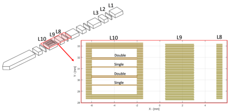
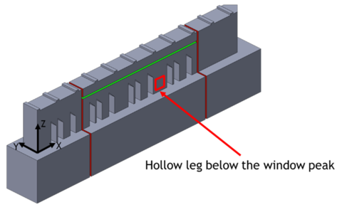
Leg L10 of each as-built part has a hollow cavity with four thin-wall structures shown in Figure 4. The outer walls of the L10 leg are approximately 0.5 mm thick and enclose two thin walls that are the width of a single laser track and another two that are the width of a double laser track. The thin walls are aligned parallel to the recoater blade direction. The bottoms of the walls sit on a solid base that is 1 mm thick, and the walls are built 4 mm high before a flat-bottomed ceiling is built. The inner regions of the L10 legs are completely sealed once the parts are built so the resulting gas and powder filled pockets preclude heat treatments until EDM cutting of the parts is completed.
2.1.4 Feedstock Material:
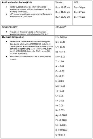
All IN718 builds were conducted using powder from a single lot and the particle size distribution (PSD), nominal powder density, and chemical composition are provided in Table 1. The powders were kept sealed in the original shipment containers until use. Virgin powder was used for each build.
Powder PSD was also measured by NIST. Samples were acquired utilizing methods outlined Sec. 7.1.2 of ASTM B215-15. PSD was measured using a commercial dynamic imaging analysis (DIA) system, with measurement method described in ISO 13322-2:2006. Details on NIST DIA-based PSD measurement method and uncertainty analysis are available in Whiting et al. 2019. A Mill Test Certification supplied by the manufacturer for the IN718 power, and NIST PSD measurement results data are available in the /Materials directory in the AMB2022-01 challenge description dataset.
2.2 Build Parameters, Scan Strategy, and Build Conditions
Builds were conducted using the NIST Additive Manufacturing Metrology Testbed (AMMT)which is a NIST-designed and built laser-processing metrology platform. Detailed references to the AMMT design, controller, and various other research may be found on the AMMT-TEMPS website. The AMMT is also a fully functional laser powder bed fusion (LPBF) AM machine, with a continuous-wave (CW) ytterbium fiber (Yb:fiber) laser, with a central wavelength of 1070 nm, directed by fully-controllable scanning galvanometer mirrors. The controlled laser scanning is synchronized to various measurement instrument triggering and data acquisition.
2.2.1 Nominal build parameters:
Table 2 gives the nominal processing parameters and conditions used during the AMB2022-01 3D builds. Scan strategy of the bridge-structure parts utilized standard hatching strategy which alternates between 90° (Y direction) for odd-numbered layers, and 0° (X direction) for even-numbered layers. Further details on scan strategy, gas flow, and substrate temperature are given below.
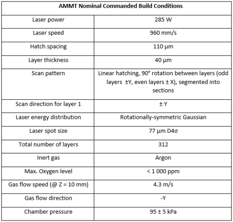
Figure 5 details the general order in which each part is scanned by the laser. Note the color bar on the left of the image, which indicates the order of laser scan via colormap. This general part-to-part order repeats for all layers.
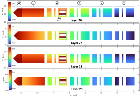
To provide similar cooling rates between the odd and even layers, the build is separated into regions that are 14 mm across along the X direction. For a given layer, the laser builds each region sequentially. Figure 6 shows the scan sequence for four layers of Part 1, starting with Layer 26 where the thin walls are first formed. Note that the starting point and scan progression within each 14 mm region changes every layer. For example, the region labelled (1) in Figure 6 progresses as follows:
- Layer 26: Horizontal scan vectors, hatches progressing in +Y.
- Layer 27: Vertical scan vectors, hatches progressing in -X.
- Layer 28: Horizontal scan vectors, hatches progressing in -Y.
- Layer 29: Vertical scan vectors, hatches progressing in +X.
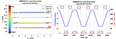
The thin-wall members that lie within Leg 10 of each part have laser scan order and timing shown in Figure 7. The order and direction each track is scanned in the thin-wall region is the same for every layer. Note that the laser ‘on’ and laser ‘off’ (e.g., skywriting) timing between tracks varies, and depends on the spacing of scan tracks and part geometry.
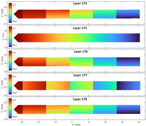
The solid part of the bridge structure starts at Layer 175 (height of 7 mm), where the gaps between legs merge. The scan strategy in the solid portion of the structure proceeds as shown in Figure 8. Note that Layer 175, immediately after the bridge legs merge, is not separated in the 6 regions as shown Figure 6.
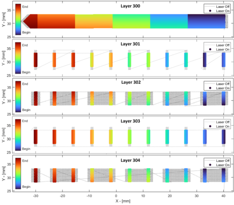
The 11 tabs on top of the bridge structure start at Layer 301, as shown in Figure 9. These are scanned in a similar sequence as the rest of the structure, grouped into same 6 regions highlighted in Figure 6. This results in each pair of tabs to be scanned together before proceeding to the next region.
2.3.1 Detailed Scan Strategy Data:
While the nominal build parameters and general laser scan strategy are described above, these do not fully define the order, timing, or position the laser scans throughout the build. The AMMT is a completely open build platform allowing us to provide unambiguous scan strategy data. The complete scan strategy for the 3D build is available as a single HDF5 file. The HDF5 and example Matlab scripts for extracting the data and creating the above plots, are available in the /Scan_Strategy/ directory of the AMB2022-01 challenge description dataset.
The HDF5 file’s /XYPT/ subgroup contains 312 numbered subgroups representing each layer’s scan strategy data (e.g., /XYPT/1/ for layer 1). Each layer subgroup then contains four vectors: X, Y, P, and T, corresponding to the digital commands executed by the AMMT. These represent the laser spot X-position in [mm], Y-position in [mm], commanded laser power in [W], and an instrument trigger (an unsigned integer). The corresponding time period between each element within the X, Y, P, and T vectors correspond to 10 μs, or a digital command rate of 100 kHz.
Note that these are the commanded positions sent to the AMMT controller, whereas the actual traversed scan position and timing may be affected by laser or galvo calibration errors (Lane et al. 2020, Yeung et al. 2020), dynamic galvo positioning error (Yeung et al. 2016), or dynamics of the laser on/off modulation (Grantham et al. 2016), though these should be minimal for most modeling purposes.
2.3.2 Gas flow system:
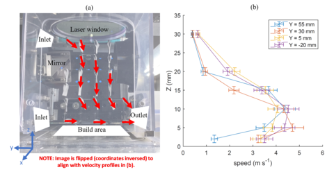
Inert gas flow across the laser melting process is used to remove process byproducts (metal vapor, condensate, and ejecta) from the laser path, build area, and chamber windows. Previous studies have shown that ineffective gas flow interferes with laser delivery and may result in powder bed contamination ( Ladewig et al. 2016, Deisenroth et al. 2021). The AMMT gas flow system incorporates a two inlet and one outlet system, as shown in Figure 10a. As shown by the orientation of the fabric tufts in Figure 10a, the inlet locations at the top and bottom of the process enclosure prevent the formation of a recirculation zone that would reduce the efficacy of byproduct transfer to the outlet.
The total flow rate of argon through the build chamber was approximately 390 L/min. This flow rate and nozzle configuration results in spatial distributions of the gas flow speed in the Y and Z directions, which are approximately invariant in the X direction across the build area. The combined speed resulting from the Y and Z velocity components of the flow was measured by hot wire anemometry at several Y and Z locations at approximately X = 0 mm to characterize the flow across the build space. Details of the speed measurement are described in Weaver et al. 2021. As shown in Figure 10b, the gas speed at the single track and pad location (near X = 0 mm, Y = 30 mm) at Z = 10 mm is approximately 4.3 m/s, which is used as a representative gas flow speed value.
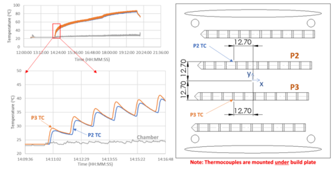
2.3.3 Build Plate Temperatures:
During the 3D builds, two type-K thermocouples were mounted under the IN718 build plate, at approximately the (-12.7 mm, -12.7 mm) position under Part 3, and (-12.7 mm, 1.7 mm) position under Part 2, as shown in Figure 11. Another thermocouple was suspended above the build area within the chamber. During the duration of the approximately 6 h build, the maximum substrate temperature increased from ambient to approximately 82 °C to 86 °C, and the chamber temperature fluctuated and rose to approximately 27 °C to 30 °C. Thermocouple measurement data are provided as columnar timeseries for builds 6, 7, and 8 in the /Thermocouples/ directory of the AMB2022-01 challenge description dataset.
2.4 In Situ Monitoring Systems
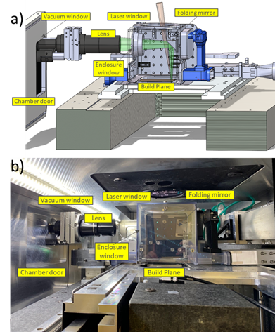
2.4.1 Staring Thermal Imaging:
Figure 12 a) shows a diagram of the staring imaging system used for in situ thermographic measurements and b) shows a photograph of the completed system. To the greatest extent possible, this system was designed to provide nearly identical layer scan patterns, measurement methods, instruments, and gas flow conditions for the sets of 3D build benchmarks (AMB2022-01 and AMB2022-02) and the 2D bare plate benchmarks (AMB2022-03).
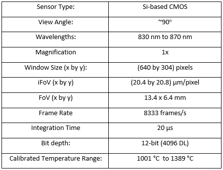
The properties of the camera used for the in situ thermography measurements are given in Table 3. Although this camera is capable of frame rates greater than 30 kHz, practical considerations limited us to 8.333 kHz for the 3D builds., which is still far better than the 1.8 kHz that was possible for AM Bench 2018. This high data rate makes it impossible to take data continuously throughout the build within the region of interest, so data were acquired using the layer scheme: 1, 2, 5, 6, 9, 10… This scheme allows direct comparison between adjacent odd-even build layers. These data have been converted into a complete spatial 3D data set by copying from nearby layers with the same laser path direction. This layer measurement scheme includes redundancy compared with the more sparse 1, 4, 7, 11… data collection scheme.
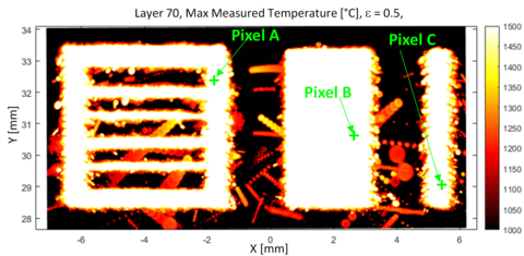
The field of view (FoV) for the in-situ thermography is marked by the red box in Figure 1-4. It encompasses the entirety of Legs 8, 9 and 10, which are split between scan sections 3 and 4 in Figure 6. The FOV is offset from the island section geometry so that the thermography captured from the small and medium legs are indicative of the nominal thermal history of the other small/medium legs.
2.5 Sample Cutting
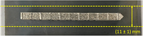
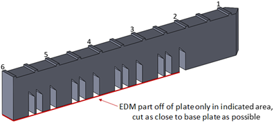
Before conducting ex situ measurements, the 4 parts on each build plate are separated from one another via EDM cutting, as shown in Figure 13. As a result, the parts used for distortion and residual strain measurements are attached to a smaller portion of build plate material than during the build. The remaining build plate material measures 100 mm ± 1 mm long, 11 mm ± 1 mm wide, and 12.5 mm thick. This is the state of the samples when measuring residual strains using synchrotron X-ray diffraction and neutron diffraction as well as the starting condition when measuring both residual stresses using mechanical methods and part deflection. Smaller samples used for microstructure and XRCT studies were also extracted using EDM.
2.6 Post-Build Thermal Processing
Metal alloy components are typically subjected to well-understood annealing and/or hot isostatic pressing treatments to achieve the desired microstructure and material behavior for a given application. This is true for almost all AM-built alloys whose microstructures generally bear little resemblance to alloy microstructures obtain through more traditional processing routes. The heat treatment selected for AMB2022-01 includes a homogenization step followed by a precipitation anneal.
2.6.1 Homogenization
Samples used for ex situ characterization or for in situ characterization during a precipitation anneal were prepared using the following steps:
- cutting using electrical discharge machining
- ultrasonic cleaning in baths of ethanol and acetone
- vacuum encapsulation including prolonged pumping to high vacuum
- annealing at 1175 °C for 1 h
- water quench
Samples that were used for in situ characterization during homogenization were prepared using the following steps:
- cutting using electrical discharge machining
- ultrasonic cleaning in baths of ethanol and acetone
- sectioning and polishing to sample dimensions required for in situ measurements (if needed)
- in situ annealing at 1175 °C for 1 h in a flowing Ar atmosphere
2.6.2 Precipitation Anneal
Samples used for ex situ characterization were prepared using the following steps
- ex situ homogenization treatment as described above
- brief ultrasonic cleaning in baths of ethanol and acetone
- vacuum encapsulation to high vacuum
- annealing at 720 °C for 16 h
- water quench
Samples that were used for in situ characterization during annealing were prepared using the following steps:
- ex situ homogenization treatment as described above
- brief ultrasonic cleaning in baths of ethanol and acetone
- sectioning and polishing to sample dimensions required for in situ measurements (if needed)
- in situ annealing at 720 °C for 16 h in a flowing Ar atmosphere
2.7 Specimen Naming Convention
Any piece of material, from a complete build plate to an individual thin wall can be used as a measurement specimen or can be used to make a specimen. The following naming convention is used for almost all AMB2022-01 specimens:
AMB2022-718-AMMT-BR-PX-LY-WZ, with R = 1, 2..., X = 1, 2, 3, 4; Y = 1,…, 12; Z = 1, 2, 3, 4
Here, “AMB2022” refers to the current round of AM Bench measurements, “718” refers to the alloy used, and “AMMT” refers to the build machine used to conduct the AM build. In the subsequent designations, B = Build plate, P = Part, L = Leg, W = Wall. The build plates (B) are numbered in the order they were built, and the bridge parts (P) and the thin walls (W) are numbered from the laminar flow side of the build plate with the sequence shown in the photograph in Figure 2, right. The legs (L) are numbered as shown in Figure 1. An example valid sample designation is
AMB2022-718-B7-P2-L10-W1.
This refers to build plate 7, part 2, leg 10, and wall 1. Samples composed of multiple legs can be designated by listing them together:
AMB2022-718-AMMT-B1-P3-L1-L2-L3.
For samples that don't fit into the above, we use this -O# suffix naming convention:
-O#, where # is the sample number, # = 1, 2, 3... and O = Other. An example is the specimen
designation:
AMB2022-718-AMMT-B6-P3-O1,
which is a small specimen cut from the bridge region used to measure the unstrained lattice parameter for synchrotron X-ray residual strain measurements.
Partial names are also valid. For example, AMB2022-718-AMMT-B6-P3 refers to the third part from build 6.
The AMB2022-01 benchmark measurements include in situ phenomena during the build process, in situ microstructure evolution during the two-step post-build thermal heat treatment, and several different types of ex situ characterization measurements including residual strain and stress measurements, part distortion resulting from partial removal from the build plate, 2D microstructure characterization, 3D microstructure characterization, averaged microstructure characterization, transmission electron microscopy (TEM), and X-ray computed tomography (XRCT). The measurement methods include:
In situ measurements during the build
- Use of in situ thermography to measure the location-dependent cooling rates of the solid material immediately after solidification (after the solidus is reached)
- Use of in situ thermography to determine the time above melting (above solidus/liquidus midpoint)
Ex situ measurements
- Residual strain and stress measurements using synchrotron X-ray diffraction, neutron diffraction, and mechanical (contour) method
- Distortion measurements comparing part geometry before and after partial cutting from the build plate
- 2D cross sections measured using a combination of SEM and optical microscopy
- a 3D volume measured using a combination of serial sectioning, optical microscopy, and SEM
- High energy X-ray diffraction
- TEM
- XRCT
Combined ex situ measurements and in situ measurements during post-build heat treatment
- Ultra-small-angle X-ray scattering/small-angle X-ray scattering/wide-angle X-ray scattering (USAXS/SAXS/WAXS)
Although not used directly for the Challenge Problems, an important design criterion for AMB2022-01 was that the 3D XRCT and serial sectioning measurements were spatially registered both with one another and with the in-situ thermography and the digital command input data files. Thus, an extensive 4D (position and time during build) multimodal, digital-twin data set exists that directly connects the build process details with melt-pool level in situ processing data, micron-scale microstructure data and few-micron XRCT measurements of local defects.
3.1 In Situ Time Above Melting
Methods for defining and extracting the location-specific ‘time above melt’ from thermographic data will largely follow those from prior AM-Bench challenges for ‘melt pool length’ (Heigel et al. 2020). Similarly, due to the relative amount of noise and complexity with 3D build thermography, certain assumptions regarding material emissivity, and liquidus/solidus temperatures will be made, as well as various data filtering or processing of the thermographic image data, with the aim of providing the most accurate measurement possible. It is also recognized that there are numerous potential algorithms for defining and calculating ‘cooling rate’ from thermographic measurements or AM simulation results. Nevertheless, the following definition is designed, not necessarily to best represent thermal features directly relatable to other phenomena (e.g., thermal energy accumulation, or microstructure evolution), but provide the simplest and most unambiguous definition for modelers to derive and compare.
The CHAL-AMB2022-01-TAM modelling challenge will utilize thermographic data collected during ‘Build 6’ from the AMMT IN718 metal 3D builds (AMB2022-718-AMMT-B6). In calculating temperatures, it will utilize similar parameters used in AMB2022-03 measurements (e.g., LPBF scanning of single lines and pads without powder). Namely, these parameters are 1) the same effective emissivity value of ϵ ≈ 0.5 derived from AMB2022-03 measurements 2) the same assumed IN718 solidus temperature of 1260 °C, liquidus temperature of 1336 °C, and mid-point of 1298 °C, and 3) the same temperature range of 110 °C below solidus temperature to define the solid cooling rate.
The following algorithm is used to calculate ‘time above melt’ (tTaM) for each pixel within the field of view of thermographic video data:
- Convert thermal video to temperature utilizing assumed ϵ = 0.5, resulting in temperature vs. time for each pixel (xi,yj) or T(xi,yj,t).
- Perform spatter removal algorithm and thresholding (to be detailed in later publications).
- For each pixel (xi,yj):
- Extract temperature vs. time profile, T(xi,yj, t)
- Identify all timepoints where T(xi,yj, t) = 1298 °C (or the assumed mid-point between liquidus and solidus temperature), by finding the intersections.
- Identify the maximum time period, max(Δti) where T(xi,yj, t) > 1298 °C. Store as tTaM(xi,yj).
- If no tTaM(xi,yj) is identified, then store as ‘not a number’ tTaM(xi,yj) = NaN, or reject this pixel from further analysis.
To clarify this process, Figure 14 shows a composite image from the high-speed thermographic video data for Layer 70, where the maximum temperature experienced by each pixel is plotted. Several example pixels are indicated, and the time vs. temperature data for Pixel B is plotted in Figure 15. Additionally, Figure 15 shows the maximum time period that pixel is above 1298 °C, which defines it’s ‘time above melt’ value.
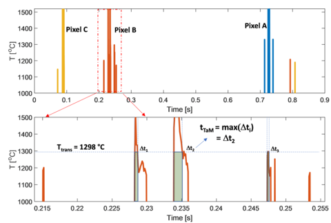
Note that while the analysis of the thermographic data will utilize an assumed Ttrans = 1298 °C, modelers using different thermodynamic material properties may wish to utilize a different temperature threshold that better represents the mid-point between liquidus and solidus of the IN718 material.
3.2 In Situ Solid Cooling Rates
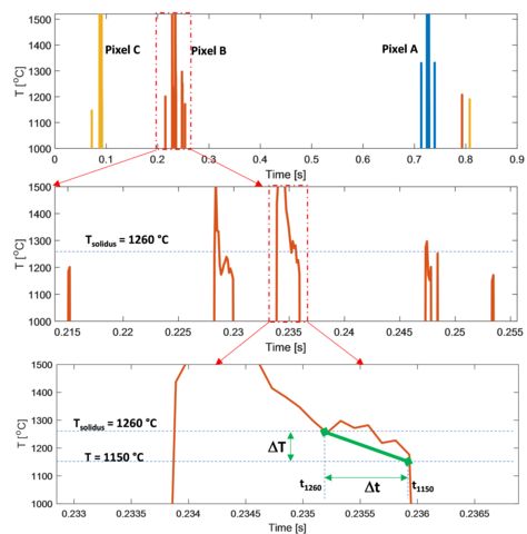
Similar to prior AM-Bench challenges (Heigel et al. 2020) and the ‘time above melt’ feature, surface cooling rates for the 3D builds will be calculated on a per-pixel basis. Additionally, similar temperature values and temperature range will be used to define ‘cooling rate’ as is used in AMB2022-03 challenges.
The cooling rate, ΔT/Δt, will be based on linear interpolation of the temperature vs. time for each pixel, T(xi,yj,t), during the same temperature peak that ‘time above melt’ was calculated. The ΔT is between the assumed solidus temperature Tsolidus = 1260 °C, and 110 °C below, resulting in fixed ΔT = 110 °C. Therefore, the objective then is to identify the time span Δt = t1260 – t1150, where t1260 is the timepoint where the temperature-time curve intersects T = 1260 °C, and t1150 where it intersects T = 1150 °C.
The following algorithm is used to extract solid cooling rate from the 3D build thermographic data:
- Convert thermal video to temperature utilizing assumed ϵ = 0.5, resulting in temperature vs. time for each pixel (xi,yj) or T(xi,yj,t).
- Perform spatter removal algorithm (to be detailed in later publications).
- For each pixel (xi,yj):
- Extract temperature vs. time profile, T(xi,yj, t)
- Identify nominal time period when ‘time above melt’ is defined (See Figure 15)
- Identify t1260 , where T(xi,yj, t) = 1260 °C (or the assumed solidus), by finding the intersection
- Identify t1150, where T(xi,yj, t) = 1150 °C, or 110 °C below the assumed solidus.
- Calculate Δt = t1260 – t1150
- Calculate SCR( xi,yj ) = ΔT/Δt = (110 °C)/Δt, and store the value
- If no SCR is identified, then store as ‘not a number’ SCR(xi,yj) = NaN, or reject this pixel from further analysis.
It is anticipated that modelers submitting results to CHAL-AMB2022-01-SCR will follow a similar algorithm and definition of SCR as described above. However, modelers are encouraged to test or implement any variation they determine as more appropriate (e.g., using a different solidus temperature), and discuss with fellow modelers and metrologists at the AM-Bench conference.
3.3 Residual Strain and Stress
Residual elastic strain (RS) within as-built IN718 parts was measured using synchrotron X-ray diffraction at beamlines 6-BM at Argonne National Laboratory’s Advanced Photon Source (APS) and 1A3 at the Cornell High Energy Synchrotron Source (CHESS), and neutron diffraction on the HB-2B High Intensity Diffractometer for Residual Stress Analysis (HIDRA) instrument at Oak Ridge National Laboratory’s High Flux Isotope Reactor (HFIR). Residual stresses within both the baseplate and an attached as-built part were measured using the mechanical contour method at the University of California Davis and Hill Engineering. Both sets of synchrotron X-ray RS measurements and the mechanical residual stress measurements were conducted on the same part, AMB2022-718-AMMT-B7-P3. The neutron diffraction RS measurements were conducted on a nominally identical part, AMB2022-718-AMMT-B7-P4. The synchrotron X-ray and neutron unstrained lattice parameter measurements were conducted using small rectangular prism specimens, AMB2022-718-AMMT-B6-P3-O1 and AMB2022-718-AMMT-B6-P3-O2, that were extracted from the bridge section of the designated part.
3.3.1 Synchrotron X-ray energy dispersive diffraction
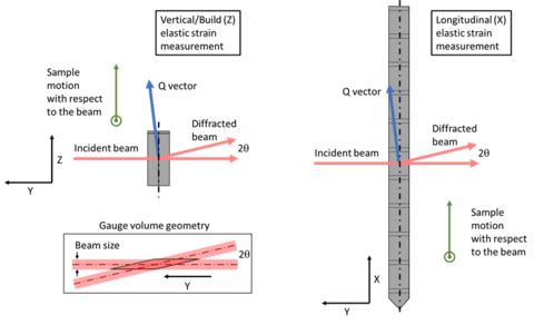
Both sets of synchrotron X-ray measurements used energy dispersive diffraction (EDD) that utilized a high energy, polychromatic X-ray beam and an energy sensitive X-ray detector at a fixed 2q angle. Figure 17 shows a generic geometry for an EDD measurement, where the incident and diffracted beam sizes are assumed to be the same.
3.3.2 Neutron diffraction
Neutron diffraction residual strain measurements typically require much large gauge volumes and data acquisition times than corresponding elastic strain measurements using synchrotron X-ray diffraction. However, neutrons are considerably more penetrating than typical high-energy X-rays and can conduct measurements along three orthogonal axes, providing improved access to stress states.
Figure 18 shows the neutron diffraction measurement geometry. The neutron diffraction measurements at HIFR used a 311 reflection to probe the 311 lattice spacings averaged over the measurement volumes in the X, Y, and Z directions. As with the synchrotron X-ray RS measurements, the gauge volume is defined by the intersection of the incident beam and the diffracted beam. For these neutron measurements, the 2 90° and the square cross section beam widths are 1.5 mm.
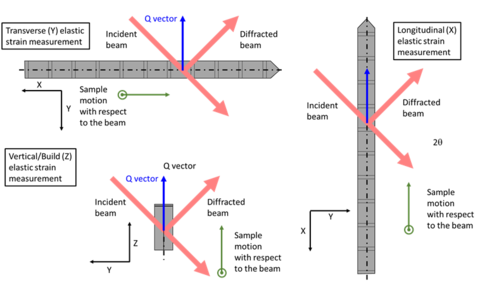
3.3.3 Contour method
A mechanical stress release technique (Prime et al. 2013) referred to as the contour method was used to measure residual stresses perpendicular to the cut planes shown in Figure 19. Thus, the YZ plane slices are used to measure σxx stress components and the XY plane slice is used to measure σzz stress components.
3.4 Part Distortion
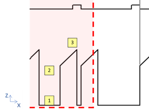
After being built, the part remains on a section of the build plate. The tops of all 11 ridges are skim cut parallel to the build plate to remove the rough as-built surface to allow for more accurate measurement. The vertical height, relative to the surrounding base plate, of every other ridge on the stop surface of the part is measured using a coordinate measurement machine (CMM). Six points are sampled on the top of each ridge to ensure coverage of the surface. To minimize the influence of the build plate warp of the measurement, the areas adjacent to the ridges are used as the reference, as shown in the drawing below. Least-squares fit features will be utilized to evaluate the measurands. These initial measurements will make up ziinitial, where i=1:6 using the numbering in Figure 20 below.
Next, the part is EDM cut such that only the end portion of the part remains attached to the plate (see Figure 21), and the cut section of the part will deflect upward from relaxation of the as-built residual stresses. The part will then be measured again per the measurement definition using a CMM, and will make up zicut.
For these benchmark comparisons, the part distortion is defined by the vertical deflections of all measured ridge edges after being cut with EDM. Thus, δi = zicut - ziinitial, where δi is the vertical deflection of edge i. The final qualitative result will be the vertical deflection of the component estimated at the center of the measurement ridge for each of the six ridges. An uncertainty value for the measured deflection will be provided and will be calculated based on substitution measurements.
3.5 2D Cross Sections
3.5.1 Measurement locations:
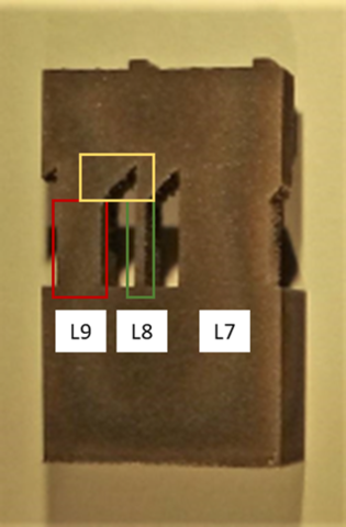
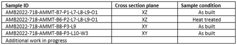
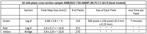
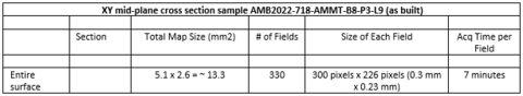
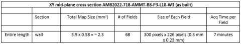
2D cross sections through the as built and heat-treated samples were examined using Scanning Electron Microscopy (SEM) methods including Electron BackScatter Diffraction (EBSD), Energy Dispersive Spectroscopy (EDS), and Large Area Mapping (LAM). The cross sections include XZ and XY planes of the solid material, and YZ and XY planes of some thin walls internal to leg L10. Figure 22 shows the XZ mid-plane cross section AMB2022-718-B7-P1-L7-L8-L9-O1 (as built). The regions outlined by the green, red, and yellow boxes designate locations of EBSD montages. The red and green regions extend at least 500 μm into the baseplate. Table 4 shows the sample IDs for the various cross sections that were measured.
3.5.2 Sample preparation:
After EDM cutting, samples were prepared by progressive polishing from 600 grit SiC paper down to 1 mm diamond suspension. Final surface preparation used vibro-polishing with 0.05 mm non-colloidal silica for 16 h. Samples were cleaned in an ultrasonic bath in three solutions: soap/water, water, and ethanol.
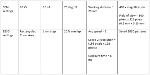
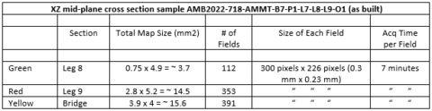
Imaging and data acquisition were performed using a JEOL Field Emission JSM7100 with the Oxford Symmetry S2 EBSD detector with fore-scatter diodes and the Oxford Ultim Max EDS 100 mm2 silicon drift detector. Oxford Aztec software Ver 6.0 was used for EDS/EBSD analysis and to create Large Area Maps. The measurement conditions are listed in Table 5. Detailed descriptions of the Large Area Maps are provided in Table 6 to Table 9. Additional large area mapping is in progress and this document will be updated as information becomes available.
3.5.4 EDS:
High spatial resolution EDS elemental mapping from limited localized sample areas is in progress and this document will be updated as information becomes available.
3.6 3D Microstructure
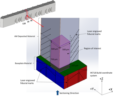
This set of automated serial sectioning measurements (Uchic et al. 2012, Chapman et al. 2021) was designed to produce a micron-scale, 3D characterization of the microstructure within a region of interest (ROI) of a 2.5 mm leg and extending into the baseplate. Figure 23 shows the 3D ROI within the base of the 2.5 mm leg AMB2022-718-AMMT-B8-P1-L9. This ROI was also within the field of view of the in-situ thermography measurements during the build process. The ROI measures approximately 500 µm × 500 µm × 750 µm along the build X, Y, Z directions respectively, and is contained in a larger needle shaped region excised from the leg using wire electrical discharge machining (EDM). All EDM cuts were separated from the ROI by at least 250 µm. Additionally, the Z dimension of the ROI includes approximately 250 µm of the baseplate material. Fiducial marks were laser engraved onto all X and Y faces of the specimens using a Micromac microPREP PROTM system, with all fiducial marks separated from the ROI by at least 50 µm. The specimens were then affixed in a specially designed holder which was incorporated into a conductive metallographic mount. The build X and Y directions lie in the plane of the mount, with the build Z direction oriented inward and normal to the mount surface.
Each serial sectioning step proceeds by first removing approximately 2 µm of material, including a final polish with 40 nm colloidal silica in a Robomet.3DTM system. The height of the serial section surface is determined for each section using a differential imaging measurement. The specimen is then transferred to a Zeiss AxioImager.Z2m optical microscope to collect several optical bright-field images, including a montage of the full cross section. Next, the specimen is transferred to a Tescan Vega 3 scanning electron microscope (SEM) where a backscatter electron (BSE) image covering the full specimen cross section is collected. This is followed by collection of a higher resolution BSE image covering a more limited field of view centered on the ROI. Finally, an electron backscatter diffraction (EBSD) image is collected with the specimen at a 70° inclination using a Bruker Quantax e-Flash 1000 EBSD detector.
The individual datasets described above are post-processed to produce a 3D reconstruction of the ROI using a range of tools including ImageJ/Fiji, DREAM.3D, and custom scripts. The individual optical montages are first reconstructed into a 3D stack by aligning features visible in the metallographic mount. Next, to minimize distortions introduced in SEM data collection, the lower resolution BSE image is spatially registered to the optical montage from the corresponding slice. Next, the higher resolution BSE image covering just the ROI is registered to the larger area BSE image, and finally the EBSD data are registered to the higher resolution BSE image. The ROI contains two orthogonal as-printed exterior surfaces as well as the top-surface of the substrate plate. These features are sufficient to locate the ROI with respect to the original build coordinate system. Application of this series of transformations therefore allows placement of ROI data into the original build coordinate system. The final ROI spans from unaffected baseplate material, through remelted baseplate material, and into additive deposited material.
3.7 Transmission Electron Microscopy
Specimens for TEM are prepared either by jet polishing or by dimpling and ion milling as appropriate. Specimens are examined first by conventional TEM techniques, such as diffraction contrast imaging and selected area diffraction to ascertain the distribution and directionality of grains, the distribution and identity of precipitates, and the presence of any frequently-occurring crystallographic defects or other features. When necessary, traditional techniques are supplemented with spectroscopy, HRTEM, and STEM to fully sufficiently characterize the materials.
3.8 X-ray Computed Tomography
Lab-scale X-ray Computed Tomography measurements were taken (using a Zeiss Xradia Versa XRM-500) of individual AMB2022-718-AMMT-B8-P1-L1 (“Leg 1” here), AMB2022-718-AMMT-B8-P1-L8 (“Leg 8” here), and AMB2022-718-AMMT-B8-P1-L10 (“Leg 10” here), after they had been mechanically separated from the rest of the workpiece. The sliver of AMB2022-718-AMMT-B8-P1-L9 (“Leg 9” here) having been exhumed via EDM (as described in Section 3.6) was also measured, before being destroyed by the measurement described in Section 3.6. These measurements provide relatively high resolution, fully 3D, nondestructive measurements of the parts, provided by density contrast. i.e., the resulting images will differentiate between metal and air/void space, enabling porosity, overall shape, surface topography, and void-type defect shape measurements.
The X-ray source voltage, power, filters, and exposure time were optimized on a case-by-case basis to achieve the highest quality images possible while maintaining as high of resolution as possible. In general, between 140 kV and 160 kV accelerating voltage along with 10 W of power and the strongest available filter were used, with required exposure times of between 6 s and 12 s. Depending on the specimen, different numbers of projection images were required as well: Legs 1, 8 and 10 used 3001 projections over 360 degrees of rotation, while Leg 9 used 2401 projections over 188 degrees of rotation.
Resolution was limited by the size of the objects: the detector has an effective width of roughly 1850 pixels (using the built-in wide mode to virtually increase the detector width), so the achievable voxel size while keeping the whole specimen in the field of view is roughly 1/1850th of the specimen’s longest cross-sectional dimension (in the case of rectangular legs, this is the diagonal). Thus, Leg 1 was measured at a voxel edge length (called pixel size by the instrument) of 5.5006 µm/voxel-edge, Leg 8 was at 6.5009 µm/voxel-edge, the extracted sliver of Leg 9 was at 2.0025 µm/voxel-edge, and finally Leg 10 was measured at 5.9996 µm/voxel-edge (note: voxels here are perfect cubes). Differences in voxel edge length enable the measurement to fully capture the leg, or part of a leg, for each of the different leg geometries. In all cases, the leg was mounted as close to vertical in the instrument as we could achieve. In order to measure the full height of the specimen, vertical stitching using the built-in machine software was used to image multiple fields of view vertically and combine them into one image. Where possible, care was taken to include unique markers or fiducials to enable cross-registration between X-ray CT data and the other data provided in this dataset.
The raw projection images were reconstructed using machine-specific proprietary reconstruction software (Reconstructor Scout-and-Scan version 14.0.14829). From this, reconstructed 16-bit grayscale images were exported as stacks of image slices roughly perpendicular to the build direction (i.e., slices perpendicular to the vertical axis of the scan). The grayscale images were processed and a threshold applied to produce binary images. This process was conducted using a collection of Python scripts that rely on a mixture of 2D and 3D SciKit-Image and OpenCV functions to apply basic filtering (e.g., non-local means, unsharp mask) and thresholding steps (single value or local/adaptive), to produce black (air) and white (metal) 3D images. Minimum detectable linear feature sizes using these techniques are generally assumed to be roughly 3 to 5 times the voxel edge length.
3.9 High Energy X-ray Diffraction
Bulk phase determination and phase fraction analyses are essential components of materials characterization. In a transmission mode, we performed high-energy X-ray diffraction (HEXRD) measurements at beamline 11-ID-B of the Advanced Photon Source, Argonne National Laboratory. We used highly penetrating monochromatic high-energy X-rays at X-ray energies higher than 58 keV. The samples have an approximate lateral dimension of 5 mm × 5 mm. The sample thickness is specimen specific. We moved each sample in the beam to ensure that all sample volumes were measured for statistical purposes. We used a 2D detector to capture the diffraction patterns to reduce the texture effect.
With a time resolution of about four minutes, the USAXS instrument at the APS uses small-angle scattering to obtain information about a sample’s microstructure over a size range from micrometers to below one nanometer while simultaneously using diffraction to probe the phases present. The instrument uses ultra-small-angle X-ray scattering (USAXS) to study the larger length scales, pin-hole small-angle X-ray scattering (SAXS) to study the smaller length scales, and wide-angle scattering (X-ray diffraction) to obtain the phase information, including the most common precipitates. Detailed information on this unique instrument and its use may be found here. These transmission measurements use thin transverse specimens cut from 2.5 mm legs. Conventional metallographic polishing methods are used to thin these specimens to approximately 35 µm. Measurements were conducted in situ during both homogenization and precipitation thermal processing.
4. Description of Benchmark Challenge Problems
4.1 In Situ Build Benchmarks
4.1.1 CHAL-AMB2022-01-TAM
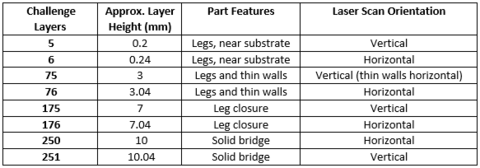
The ‘time above melt’ modelling challenge will be based on eight individual selected layers from the 3D build that span the general range of geometric features and laser scan directions. Figure 24 gives an outline of the eight layers that will be used in the challenge, and Table 10 provides more detail.
Modelers are to calculate ‘time above melting’ as close as possible to the definition or algorithm described in Section 3.1. After extracting ‘time above melting’ values, modelers should select TaM values from a region that is nominally commensurate with the in situ thermal camera field of view. From these extracted TaM values, and for each of the 8 layers, modelers should calculate the following statistical features for the CHAL-AMB2022-01-TAM modelling challenge:
- Number of pixel/element/nodes that TaM is interrogated from model results (e.g., sample size)
- Mean of all pixel/element/nodal TaM values
- Median of all pixel/element/nodal TaM values
- Standard deviation of all pixel/element/nodal TaM values
Additionally, modelers should supply pictures and/or a brief description of the model formulation (e.g., finite element, finite difference, boundary element, etc.) and visualizations of results. These will be used by AM-Bench organizers to select and request submission of invited papers to a special journal issue. Finally, modelers may wish to provide modelled and tabulated full TaM results array data to AM-Bench organizers, along-side the above-mentioned statistical features, which may be used for more comprehensive statistical comparison to thermographic results, as an example and for discussion during the AM-Bench conference.
Note that it is not expected that the AM simulation outputs exactly replicate the temporal, spatial, or temperature resolution or range of the thermographic imaging system, and model formulations may utilize certain approximations that render results outputs that are less-physically equivalent to the thermographic measurements described in Section 3.1. Therefore, participants should consider the following:
- The number of pixels/elements/nodes may vary, but should not be more than N = 1E6 (e.g., equivalent to approx. 5 μm pixel size). Additionally, values should be extracted from a uniform grid on the surface of each layer so as not to weight the statistics towards certain regions.
- In calculating the above statistical features, modelers should reject values outside the measurable/calculable TaM results (e.g., reject ‘0’ values). Modelers may also wish to reject statistical outliers.
- Depending on the model formulations, modelers may also consider testing or utilizing different algorithms or definitions of ‘time above melt’ (e.g., using a different threshold temperature). However, for the modelling challenge, model results will be compared against measurement results as described in Section 3.1. Only one entry from each participating research group will be used for the challenge judging.
4.1.2 CHAL-AMB2022-01-SCR
Modelers are to calculate the ‘solid cooling rate’ (SCR), as close as possible to the definition or algorithm described in Section 3.2, for the same layers to be modelled for the ‘time above melt’ challenge described in Table 10. After extracting SCR values, modelers should select values from a region that is nominally commensurate with the in situ thermal camera field of view. From these extracted SCR values, and for each of the 8 layers, modelers should calculate the following statistical features for the CHAL-AMB2022-01-SCR modelling challenge:
- Number of pixel/element/nodes that SCR is interrogated from model results (e.g., sample size)
- Mean of all pixel/element/nodal SCR values
- Median of all pixel/element/nodal SCR values
- Standard deviation of all pixel/element/nodal SCR values
Additionally, modelers should supply pictures and/or a brief description of the model formulation and visualization of results as described above for the CHAL-AMB2022-01-TAM challenge, and consider providing tabulated SCR results data to AM-Bench organizers. Further notes and considerations described above for the CHAL-AMB2022-01-TAM challenge are also applicable to the *-SCR challenge.
4.2 Ex Situ Benchmarks
4.2.1 CHAL-AMB2022-01-RS
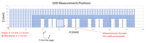
Although elastic strains and stresses were characterized using synchrotron X-ray diffraction at both the APS and CHESS, neutron diffraction at HIFR, and the contour method by UC Davis and Hill Engineering, the CHAL-AMB2022-01-RS challenge problem will specifically target only the CHESS measurements on part AMB2022-718-AMMT-B7-P3. Figure 25 shows the 2248 synchrotron X-ray sample measurement positions in the XZ plane for the part. The sampled volume was centered on the midplane of the part along the Y axis as described above in section 3.3. Elastic strains in both the X and Z directions were measured for each sample location. The challenge problem submission template can be downloaded from the /ChallengeSubmissionTemplates/ directory of the AMB2022-01 challenge description dataset. Columns 1, 2, and 3 provide the nominal X, Y, and Z coordinates for each sample location. The X and Z origins are specified in Figure 25, and the origin for Y is defined as the plane closest to the reader based on Figure 25. The mid-plane of the sample has a value Y = + 2.5 mm. The predicted XX elastic strain (exx) should be inserted into Column 4 and the predicted ZZ elastic strain (ezz) should be inserted into Column 5. Participants may use any method they like to predict the strains at the specified sample coordinates, but it is important to note that the measured values we will be comparing with are volume averages as described in section 3.3. Note that although measurements were made through the hollow thick leg that contains the thin walls and powder, no strain predictions are necessary for those positions and these have been marked on the provided template.
4.2.2 CHAL-AMB2022-01-PD
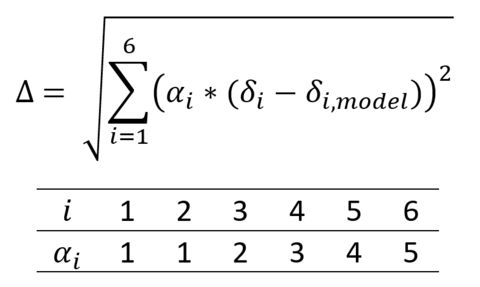
The δi will be measured for the six ridges investigated and modelers should attempt to extract similar information from their models by estimating the deflection for each ridge perpendicular to each feature’s respective datum at the center of the measurement ridge. Modelers should provide a δi for each of the of the six ridges described rounded to three significant digits (e.g. X.XXX mm). Modelers will be judged by calculating the RMS error between the modeled and measured deflection values using a weighted constant, αi, which gives higher weight to the struts on a longer portion of unsupported material (i.e., the point of greatest anticipated deflection). This metric and the values for αi are given below
4.2.3 CHAL-AMB2022-01-MS
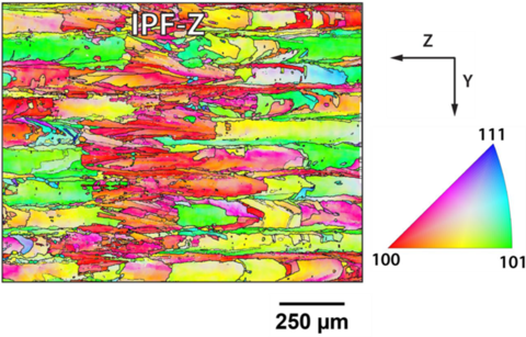
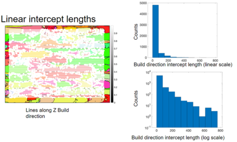
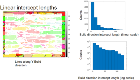
There are many possible metrics that can be used to evaluate the degree of similarity between measured and simulated microstructures. For this challenge problem, we needed a metric that could be easily implemented by the modelers and that would readily distinguish between different directions in the microstructure. We tried several different metrics using published microstructure data from AM Bench 2018 IN625 builds and the algorithm we selected is a histogram of chord lengths obtained from multiple parallel lines intersecting grain boundaries along the orthogonal directions. As an example, Figure 26 shows a Z-direction inverse pole figure (IPF) map obtained using EBSD from a YZ surface within an AM Bench 2018 IN625 build (refer to Figure 9 in 2018 measurement description). Here, adjacent pixels with a 2° misorientation angle are delineated by a thin line, and those with an angle of 10° or higher are delineated by heavier lines. Looking only at the 10° or higher boundaries, Figure 27 shows a set of lines drawn parallel to the Z axis for a sub-region of the full measurement. Histograms of the intercept lengths are shown in both linear and log scale plots. Figure 28 shows this same analysis applied along the Z direction. Note the differences in the histograms for the two orientations.
The measurement data used for this challenge problem are the extended XZ-plane large area EBSD maps acquired from AMB2022-718-AMMT-B7-P1-L7-L8-L9-O1 (as built) and AMB2022-718-AMMT-B6-P2-L7-L8-L9-O1 (heat treated) as described in section 3.5.3. Three 1 mm x 1 mm square regions from the as built sample and two 1 mm x 1 mm square regions from the heat-treated sample will be used for the challenge problem. As shown in Figure 29, these include a region at the base of a 2.5 mm leg, a second region toward the top of the same 2.5 mm leg, and a third region within the bridge section. Using the same coordinate system described in Figure 25, the corners of the challenge regions are given in Table 11 and Table 12. The locations and sizes for regions 1 and 2 are identical for the as built and heat-treated specimens.
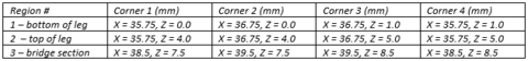

For this challenge problem, adjacent pixels with at least a 10° misorientation angle define a grain boundary. The line spacing between the parallel lines should be 5 mm and the width of the bins for the linear intercept length histograms should be 100 mm. Thus, the number of intercept lengths within the range (0,100] will be summed in the first bin, the number of intercept lengths within the range (100,200] will be summed in the second bin, etc. up to the final bin where the range is (900,1000]. It is important to note that these regions reside in the XZ plane, which is different from the AMB2018 example shown above in Figure 26 through Figure 28. The submission template for this challenge problem may be found in the /ChallengeSubmissionTemplates/ directory of the AMB2022-01 challenge description dataset. Please also submit an IPF-Z map for each sample region for which a histogram is submitted.
To participate in this challenge problem, you do not have to submit simulation results for all five requested regions. You may submit results for any or all of the regions, but the number of simulated regions will be considered in the judging.
4.3 In Situ Heat Treatment Benchmark (includes as built and final heated conditions)
4.3.1 CHAL-AMB2022-01-PE
This challenge problem is to predict the formation and evolution of phases and phase fractions, including major precipitates, as a function of time for heat treatments of IN718 within a 2.5 mm leg. As described above in sections 2.6.1 and 2.6.2, the two-step heat treatment consists of a homogenization anneal at 1175 °C for 1 h followed by a water quench, and then a precipitation anneal at 720 °C for 16 h followed by a water quench. The submission template for this challenge problem is found in the /ChallengeSubmissionTemplates/ directory of the AMB2022-01 challenge description dataset, and the corresponding measurements are described in section 3.10. The top section of the template asks for a list of all phases that are predicted to be present throughout the entire heat treatment, from as built to fully heat treated. The second section of the template asks for the predicted volume fractions for each of these phases throughout the homogenization heat treatment with a time resolution of 12 min. If a phase is not predicted to exist, please enter 0 for the volume fraction. The third section of the template asks for the predicted volume fractions for each of the phases throughout the precipitation anneal with a time resolution of 24 min. The time dependent sizes and shapes of growing or shrinking precipitates is not requested.
5. Description and Links to Associated Data
All data available to support the AMB2022-01 challenges are contained in the “AM Bench 2022 3D Build Modeling Challenge Description Data (AMB2022-01)” dataset: navigate to https://doi.org/10.18434/mds2-2607.
New data files, updates, and/or changes to download URLs may be made periodically. Users should refer to the README text file which will record all updates. Additionally, the NIST Public Data Repository (PDR) undergoes frequent updates. If file downloads fail or are unavailable, users should wait several hours before contacting the technical support listed on the AMB2022-01 dataset webpage.
Citations are provided throughout this document as hyperlinked URLs to the associated digital object identifier (DOI). Clicking these hyperlinked text should open the associated publication or cited source.
Disclaimer
The National Institute of Standards and Technology (NIST) uses its best efforts to deliver high-quality copies of the AM Bench database and to verify that the data contained therein have been selected on the basis of sound scientific judgment. However, NIST makes no warranties to that effect, and NIST shall not be liable for any damage that may result from errors or omissions in the AM Bench databases.
Certain commercial equipment, instruments, or materials are identified in this paper in order to specify the experimental procedure adequately. Such identification is not intended to imply recommendation or endorsement by NIST, nor is it intended to imply that the materials or equipment identified are necessarily the best available for the purpose.