Maps of Non-hurricane Non-tornadic Extreme Wind Speeds for the Contiguous United States
Summary
The goal of this project is to propose a new set of maps of extreme wind speeds for the next revision of Minimum Design Loads for Buildings and Other Structures which is published by the American Society of Civil Engineers. Since high winds exert great forces on structures, especially tall buildings, the maps are necessary for design purposes. The NIST focus was on non-hurricane and non-tornadic winds, for which all estimation is based only on measured wind speeds. Hurricane winds require other considerations and were handled by our collaborators at Applied Research Associates. Tornadic winds are not considered in these maps. The NIST challenge is to provide estimated wind speeds (non-hurricane and non-tornadic) with specified mean recurrence intervals between 10 and 100,000 years at any coordinate in the United States. A wind speed such that the probability of a gust with its magnitude or greater happening in any given year being 1/N has a mean recurrence interval of N. These wind speeds are also referred to as N-year return values. Such maps are possible because there exists a network of meteorological stations throughout the contiguous United States that record the speed of high winds when they occur.
The maps are constructed in two stages. In the first stage, an extreme value model is fitted to the measured wind speeds from each station. This fitted model is used to estimate the return values of interest. The model is a two dimensional Poisson process for exceedances of a high threshold as described by Smith (2004). In the second stage the maps are created by smoothing the estimated return values using local regression (Cleveland and Devlin, 1988). Standard errors and point-wise confidence intervals are based on the smoothing.
RELATED PROJECTS:
Description
DESCRIPTION:
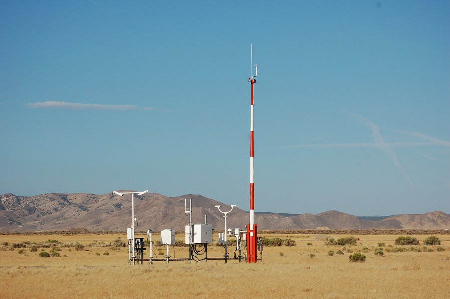
The Automated Surface Observing Systems (ASOS) meteorological station at Milford, Utah is pictured below (original image from http://www.wrcc.dri.edu/images/Station_pics/Utah/milford_ut_asos.jpg).

The instrument that measures wind speed is the red and white striped pole. Since the purpose of the maps is to display estimated values of extreme winds, only wind speeds above a minimum threshold are used in their creation. The minimum wind speed can change slightly from station to station, but it is often about 30 miles per hour (mph). The units of mph are used instead of the international system of units (SI) meters per second because the final maps will be published in units of mph. The stations also have the ability to differentiate between winds originating from thunderstorms and those that do not.
Data
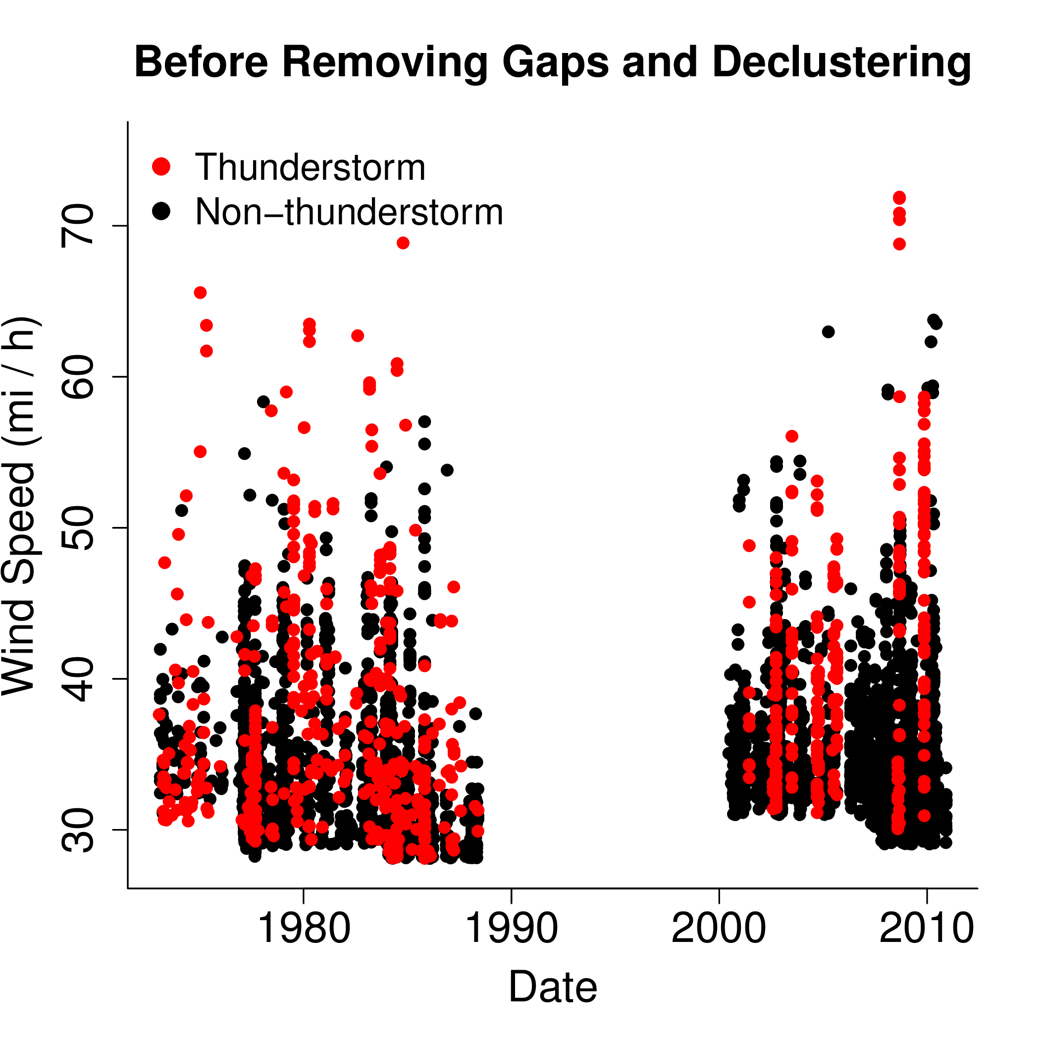
In the figure below, the raw data from an example station is depicted.

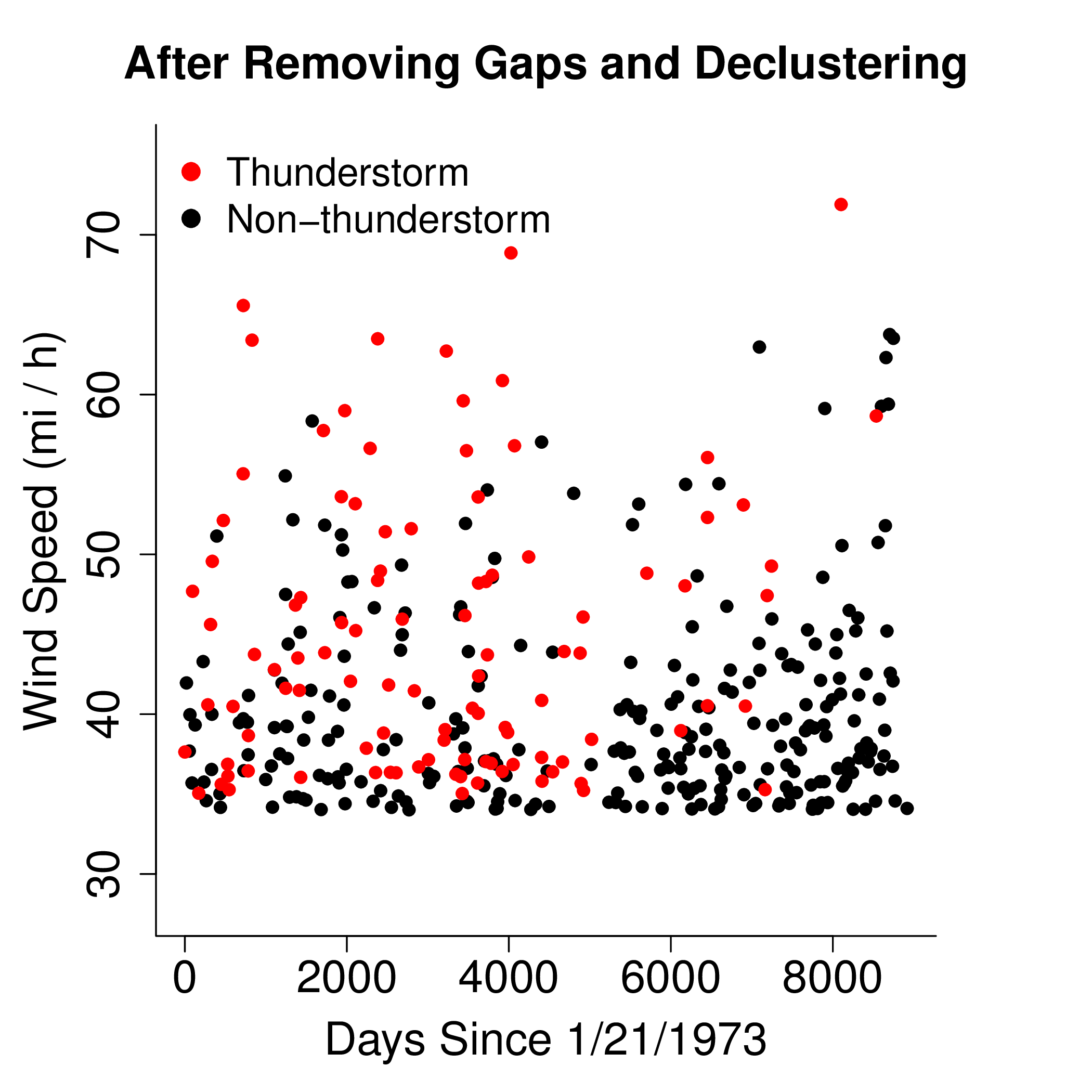
The raw data from the example station nicely illustrates several challenges that we faced. First, the threshold used in data collection not only changes between stations, but it also changes from time to time within the same station (always around 30 mph). This turns out not to matter because alternate, higher thresholds are selected during the fitting process to optimize the fit of the model to the data. Second, the observations cluster together, which is inappropriate for the Poisson process model. The clustering phenomenon makes physical sense because the underlying atmospheric conditions that result in strong winds may persist for hours in the case of thunderstorms to days in other cases. The clustering phenomenon is easily removed before fitting by identifying the clusters and using only cluster maximums for estimation. Last, there can be long spans of time (years) in which no observations are recorded. This is inconsistent with our expectations and observations. Multiple wind speeds of over 30 mph should be recorded within a year at most locations in the United States. It is unconservative in terms of estimating the N-year return values to assume that the station was working properly during this time but that there were no strong winds. So, all time spans of six months or more in which no wind speeds are recorded are removed from the raw data. This changes the definition of time from an absolute date to the amount of time that has past since the first observation was recorded. The figure below depicts the same raw data as before, but after choosing higher thresholds, declustering, and removing the observation gaps. Notice that thunderstorm and non-thunderstorm winds may have different thresholds.

It is also necessary to include a roughness correction since not all stations are sited in flat, open fields like the one in Milford. That correction is described by Masters et al. (2010).
Poisson Process
The two dimensional Poisson process used to model the extreme winds at each station is described by Smith (2004). The model has six parameters, three each for the thunderstorm and non-thunderstorm wind speeds. The three parameters are interpreted as location, scale, and tail length. The maps proposed to the committee revising the standard use a set tail length of zero. This corresponds to modeling yearly maximum wind speeds by a Gumbel distribution, which is often done. Negative values of the tail length parameter indicate a finite tail length, i.e., a maximum possible wind speed. Nonnegative values indicate and infinite tail with larger values putting more probability at higher wind speeds. The fitted Poisson process models may be used to estimate the N-year return value for any N.
Smoothing
The maps are created by smoothing the estimated return values using local regression (Cleveland and Devlin, 1988). A first degree local polynomial is used for all maps. The neighborhood size is adaptive encompassing a fixed proportion of the stations. It is chosen by incrementally increasing the neighborhood size, starting at the value indicated by generalized cross validation until a map of sufficient smoothness—as judged by the subject matter experts—is found. The fit of the smooth surface to the estimated return values is judged by examination of residuals.
Results
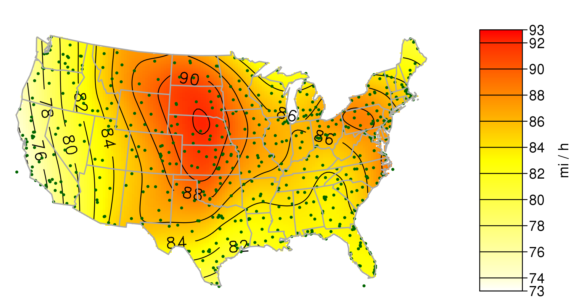
The results for N=50 are found in the figure below. There is a peak in the center of the country and a gradual decline toward the west coast. A smaller decline is observed in the north of Maine and the gulf coast. Recall that these maps do not include hurricane winds, but the final maps in the standard will. The points indicate the location of the stations that were used.

References
R. L. Smith (2004) Statistics of Extremes, with Applications in Environment, Insurance, and Finance, in Extreme Values in Finance, Telecommunications, and the Environment, eds. Bärbel Fin>nkenstädt and Holger Rootzén, Chapman & Hall/CRC.
W. S. Cleveland and S. J. Devlin (1988) Locally-Weighted Regression: An Approach to Regression Analysis by Local Fitting. Journal of the American Statistical Association, 83, 596 – 610.
F. J. Masters, P. J. Vickery, P. Bacon, and E. N. Rappaport (2010) Toward objective, standardized intensity estimates from surface wind speed observations. Bulletin of the American Meteorological Society, 91, 1665 – 1681.
Major Accomplishments
- (Draft technical report) A. L. Pintar, E. Simiu, M. Levitan, F. Lombardo, Maps of Non-hurricane Non-tornadic Wind Speeds with Specified Mean Recurrence Invervals for the Contiguous United Stated Using a Two-dimensional Poisson Process Extreme Value Model and Local Regression.
- (R package) The each map is stored as a table with four columns (longitude, latitude, estimate, and standard error). It was necessary to create software to display the maps as well as perform interpolations "on the fly" when estimates are sought at coordinates not in the static table. An R package provided a convenient way to store and share the maps and software.
- (Presentation) A. L. Pintar and E. Simiu, Development of Extreme Non-hurricane Wind Speed Maps for Structural Design from Meteorological Station Measurements in the Contiguous United States, presented at the Fall Technical Conference in Richmond, Virginia on October 3, 2014.
- (Presentation) A. L. Pintar and E. Simiu, A Two Stage Approach to Mapping Extreme Non-hurricane Wind Speeds over the Contiguous United States, presented at the European Network for Business and Industrial Statistics conference in Linz, Austria on September 23, 2014.
- (Book Chapter) A. L. Pintar and F. T. Lombardo (2013) Mapping Return Values of Extreme Wind Speeds in Risk Assessment and Evaluation of Predictions, eds. M-L. Ting, M. Gail, R. Pfeiffer, G. Satten, T. Cai, and A. Gandy, Springer.

