A-AMB2022-01 Benchmark Challenge Problems

Share

Modelers are invited to submit simulation results for any number of challenges they like before the deadline of 23:59 (ET) on April 22, 2022 Tabulated results using the provided templates are required. Modeling results may be submitted AMBench [at] nist.gov (subject: Asynchronous%25AM-Bench%20Modeling%20Results) (here).

A Q&A webinar was held on January 28 and a recording of the presentation is available here. All questions that were asked, along with questions received by email, have been compiled into an FAQ.

All evaluations of submitted modeling results will be conducted by the AM-Bench 2022 organizing committee. There will be four separate awards made with the grouping of the challenges into award categories listed below. Award plaques will be awarded at the discretion of the organizing committee.

A-AMB2022-01: Melt pool and laser coupling dynamics during high-power laser interactions with a bare metal surface.

Award #1 – Laser coupling for a stationary laser spot
- Spot Time Dependent Absorption (CHAL-A-AMB2022-01-Spot-TDA): Predict the amount of laser light absorbed during laser irradiation for a laser spot as a function of time. See section 3.1.1 for details.
- Spot Average Absorption (CHAL-A-AMB2022-01-Spot-AA): Predict the average absorption for a laser spot both before and during keyhole formation. See section 3.1.2 for details.
Award #2 – Melt pool geometry for a stationary laser spot
- Spot Time Dependent Width (CHAL-A-AMB2022-01-Spot-TDW): Predict the melt pool width for a laser spot as a function of time. See section 3.1.3 for details.
- Spot Average Solidification Rate (CHAL-A-AMB2022-01-Spot-ASR): Predict the average solidification rate of the melt pool after laser off. See section 3.1.4 for details.
Award #3 – Laser coupling for a scanning laser spot
- Scan Time Dependent Absorption (CHAL-A-AMB2022-01-Scan-TDA): Predict the amount of absorbed laser light as a function of time during a linear laser scan. See section 3.2.1 for details.
- Scan Average Absorption (CHAL-A-AMB2022-01-Scan-AA): Predict the average absorption during a scanned laser both before and during keyhole formation. See section 3.2.2 for details.
Award #4 – Melt pool geometry for a scanning laser spot
- Scan Maximum Width and Depth (CHAL-A-AMB2022-01-Scan-MWD): Predict the maximum melt pool width and depth during a linear laser scan. See section 3.2.3 for details.
- Average Solidification Rate (CHAL-A-AMB2022-01-Scan-ASR): Predict the average solidification rate after a linear laser scan has finished. See section 3.2.4 for details.

Overview and Basic Objectives
Experiment Description
Description of Benchmark Comparisons
Data to be Provided
Relevant References

_____________________________________________________________________________________

1. Overview and Basic Objectives

The asynchronous AM-Bench 2022 challenge is to accurately model laser interaction with a melt pool during processing conditions similar to those found in laser powder bed fusion additive manufacturing. The primary objective is to determine the laser energy coupling during the given processing conditions for both a stationary and linearly scanned laser beam.

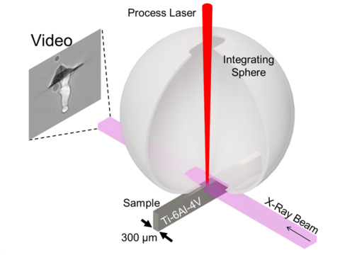
Experimental data for model calibration and challenge comparison is provided by simultaneous measurements of high-speed X-ray radiography and integrating sphere radiometry. Figure 1 shows an example of the instantaneous projected melt pool image from X-ray radiography along with the measured absorption from integrating sphere radiometry. Example videos of these data can be found in the links given at the end of this page. These experiments were carried out at the Advanced Photon Source of Argonne National Laboratory with a diagram of the experiment shown in Figure 2. Released calibration data was performed on NIST standard reference material (SRM) Ti-6Al-4V. Calibration data are available for download here and include both stationary and scanned laser data in the form of X-ray images and tabulated time-resolved absorptance data.

The data made available for model calibration is for a stationary and scanned laser on bare Ti-6Al-4V. Some of these data have been published previously. The blind modeling challenge will be to accurately predict laser energy absorption and melt pool behavior during laser processing of a bare aluminum alloy. Experimental X-ray radiography and absorption data for aluminum has not previously been released and will only be available after the challenge submission deadline. The appropriate experimental configuration necessary to model these experiments is described below.

2. Experiment Description

Specific experimental details for the calibration data given in this record can be found in a previous publication, with only a brief description provided here. General information about the development of integrating sphere radiometry for laser processing can be found here. For general information about the X-ray imaging technique, please see this publication. All calibration and challenge data were obtained at the 32-ID-B beamline of Advanced Photon Source at Argonne National Laboratory. The experimental configuration is given in Figure 2.

2.1 Integrating Sphere Radiometry

To measure the absorptivity, a custom-made, calibrated integrating sphere was placed over the metal sample to collect the backscattered laser light during laser processing. The amount of absorbed laser power is determined from an energy balance calculation between the measured input and scattered laser light (zero light transmission). The sphere had an elongated inlet aperture at the top to allow for a scanned process laser. A small channel along the sphere base accommodated clear passage of the 2-mm wide X-ray beam. The process laser had an angle of incidence of 7° relative to the sample surface normal. This ensured that the strong backscattered light from the initially solid surface would be captured by the sphere. The backscattered light was measured by a photodiode that was fiber-coupled to the sphere surface; it was bandpass filtered at 1070 nm to pass the incident laser wavelength. The photodiode voltage was measured by a high-speed oscilloscope with 40 ns time resolution. A calibration procedure using a well-characterized scattering surface in place of the experimental target produces a coefficient that converts the photodiode signal to an absolute amount of scattered light power. This procedure was repeated between laser injections so that changes to the internal surface of the sphere with time could be accounted for. Over the course of these experiments, the loss within the sphere changed only slightly, increasing on average by 0.6 % per laser exposure. The dynamic absorptance is determined by calculating the difference between the backscattered and input laser powers and then dividing by the input laser power. Normalizing this to 100 gives the percent absorption.

2.2 X-ray Radiography

The high-speed X-ray imaging experiments were performed similar to those described previously. All calibration and challenge X-ray videos were captured at 50,000 frames per second with a 2.5 μs exposure time. Both raw and processed images are provided with the image analysis description described in a previous publication.

2.3 Laser Processing Conditions

The process laser was a 1070 nm wavelength Yb-doped fiber. The beam profile at the sample surface for all simultaneous X-ray and absorption measurements was calculated to have a diameter (1/e² value) of 122.5 μm ± 3.0 μm. This is based on beam profile measurements made at multiple heights, with measured minimum spot size (beam waist) of 49.5 μm ± 5 μm. The beam profile data measured at beam focus are provided, which is not the exact location of the sample surface. The X-ray and absorption measurements were performed with the sample 2.8 mm below the beam waist, resulting in the calculated 122.5 μm spot size. The beam profile is approximately Gaussian over the range that was measured with only a slight ellipticity of greater than 92 %. A galvanometer scanner that maintains a 7° angle of incidence of the process laser beam to the sample surface is used for controlling the laser duration and scanning. The scanned challenge data had a scan speed of 700 mm/s where a "Sky-write" scan strategy was used. This ensured that the scan speed was constant the entire time the laser was on. The temporal laser pulse information is given with the tabulated absorptivity data and was approximately 2 ms long. The sample and integrating sphere apparatus were placed in an inert gas chamber with two Kapton windows that allowed for transmission of the X-ray beam. This chamber was vacuum pumped and backfilled with argon to room pressure.

2.4 Materials

The material used for the released challenge data was Ti-6Al-4V samples machined from NIST Standard Reference Material 654b using wire electric discharge machining. These were thinned to 300 μm by polishing of the sides to which the X-ray beam was incident. This thickness was necessary for adequate X-ray transmission at the high frame rate (50,000 frames per second) X-ray imaging used here. The polished sides also created a highly specular surface, which is necessary for good contrast of keyhole and melt pool in the X-ray images. The laser incident surface was also polished to a specular finish. Please see additional information for a sample diagram and more information.

[SBJ(1]This link has been changed to https://data.nist.gov/od/ds/mds2-2525/Sample%20Diagram_V110.pdf

3. Description of Blind Challenge Problems

The blind challenge will be to predict laser absorption and melt geometry during laser irradiation of bare plate aluminum. The experimental data used for comparison will be similar to that described above. The material used for the blind challenge problem is NIST SRM 1241c, which is a 5182 aluminum alloy. These samples were 1 mm thick in the direction of X-ray transmission.

3.1. Spot on Aluminum bare plate

The first challenge is for a stationary laser illumination of a bare aluminum plate. The laser duration was 1.982 ms with the sample surface placed 2.8 mm below the focus of the laser beam where the laser beam profile was calculated to be 122.5 μm. The laser power was 501 W continuous with the temporal pulse profile provided in the submission template for Time Dependent Absorption. The incoming laser beam is 7 degrees from normal incidence.

3.1.1 Time Dependent Absorption (CHAL-A-AMB2022-01-Spot-TDA)

This challenge is to predict the amount of laser light absorbed during laser irradiation. A table is provided (“Al_Spot_TDA.csv”) for the participant to submit their results. The first two columns are populated with time in seconds and applied laser power in watts, respectively. The time interval is 40 ns with time zero being the start of a 1.982 ms laser irradiation. The last two blank columns are for the absolute absorption in watts and relative absorption as a percent. The root mean squared error between the submitted prediction and experimental data will be used to determine accuracy.

3.1.2 Average Absorption Before and During Keyhole (CHAL-A-AMB2022-01-Spot-AA)

We also ask that the participant calculate the average absorption both before and during keyhole formation, as well as the standard deviation of the absorption during keyhole formation. The start of keyhole is defined as the point in time when the relative absorption is equal to or greater than 35%. An empty table is provided for the participants to populate with their results.

3.1.3 Time Dependent Melt Pool Width (CHAL-A-AMB2022-01-Spot-TDW)

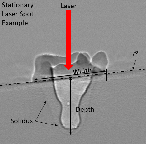
The melt pool width versus time is determined from experimental high-speed X-ray imaging data only during the time that the laser is on. For the exact temporal laser power profile, see the template provided for 3.1.1. The width is measured at the original plane of the sample surface as shown in Figure 3. A table is provided that provides a column for time in 20 μs intervals next to a blank column to be populated with the melt pool width in μm.

3.1.4 Average Solidification Rate (CHAL-A-AMB2022-01-Spot-ASR)

The solidification rate is also determined from experimental high-speed X-ray imaging data. This is calculated from the time rate of change of the melt pool depth once the laser has turned off. The melt pool depth is taken as the normal distance from the furthest solidus interface from the original surface plane as shown in Figure 3. The melt pool depth is measured in 20 μs intervals due to the frame rate of the X-ray imaging (2.5 μs exposure time). A single solidification rate is defined as the change in depth at each time interval and dividing by 20 μs, which is repeated until the melt pool has completely solidified. These values are then averaged to provide a single value for the solidification rate in units of m/s. This value can be entered in the table provided.

3.2. Scan on Aluminum bare plate

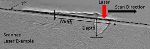
These blind challenges are similar to those described in 3.1 except with a scanning laser source. The laser power is 473 W for 1.980 ms linearly scanned at 700 mm/s. The laser is again incident to the sample surface at 7 degrees from normal with the sample positioned 2.8 mm below the focal plane where the beam diameter is 122.5 μm. Figure 4 shows the geometry and relevant definitions.

3.2.1. Time Dependent Absorption (CHAL-A-AMB2022-01-Scan-TDA)

A table is provided (“Al_Scan_TDA.csv”) for the participant to provide their results for the absorbed laser power versus time. The first two columns are populated with time in seconds and applied laser power in watts, respectively. The time interval is 40 ns with time zero being the start of a 1.980 ms laser irradiation. The last two blank columns are for the absolute absorption in watts and relative absorption as a percent. The root mean squared error between the submitted prediction and experimental data will be used to determine accuracy.

3.2.2. Average Absorption Before and During Keyhole (CHAL-A-AMB2022-01-Scan-AA)

Again, we ask that the participant calculate the average absorption both before and during keyhole formation, as well as the standard deviation of the absorption during keyhole formation. The start of keyhole is defined as the point in time when the relative absorption is equal to or greater than 25%. An empty table is provided for the participant to populate with their results.

3.2.3. Maximum Melt Pool Width and Depth (CHAL-A-AMB2022-01-Scan-MWD)

For the scanned laser challenge, we only ask for the maximum melt pool width and depth. The melt pool width is defined as the lateral distance along the original metal surface between solidus interfaces. The depth is defined as the deepest solidus interface measured relative to the normal distance to the original metal surface. These definitions are shown in Figure 4. Participants can submit their values in the template provided.

3.2.4. Average Solidification Rate (CHAL-A-AMB2022-01-Scan-ASR)

The solidification rate is determined from experimental high-speed X-ray imaging data from the time rate of change of the melt pool depth once the laser has turned off. The melt pool depth is taken as the normal distance from the furthest solidus interface from the original surface plane. This is marked in Figure 4. The melt pool depth is measured in 20 μs intervals due to the frame rate of the X-ray imaging (2.5 μs exposure time). Single solidification rates are calculated at each time interval by calculating the change in depth and dividing by 20 μs. These are then averaged in order to provide a single value for the solidification rate in units of m/s. This value can be entered in the table provided.

4. Data to be Provided

The following data will be provided on January 21, 2022 to assist in the development of models and simulations. The blind challenge submission deadline is 23:59 (ET) on April 22, 2022 with the corresponding measured data released April 25, 2022. The entire challenge problem dataset, as well as additional information about the data, are available for download here. Below are direct links to some of the downloadable materials along with a brief description.

5. Relevant Publications

Manufacturing and Materials

Additive Manufacturing Benchmark Test Series (AM-Bench)

A-AMB2022-01 Benchmark Challenge Problems

Share