
Official websites use .gov
A .gov website belongs to an official government organization in the United States.
Secure .gov websites use HTTPS
A lock (
) or https:// means you’ve safely connected to the .gov website. Share sensitive information only on official, secure websites.
AMB2018-01 Description
2018 AM-Bench Test Descriptions for AMB2018-01
Class 1 benchmark tests:
AMB2018-01: Laser powder bed fusion builds of 3D metal alloy test objects with multiple types of in-situ and ex-situ measurements. Primary focus is on residual stress, distortion, and microstructure.
- Overview and Basic Objectives
- Experiment Description
- Description of Benchmark Comparisons
- Data to be Provided
1. Overview and Basic Objectives
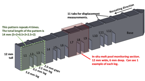
The AMB2018-01 tests consist of laser powder bed fusion (LPBF) 3D metal alloy builds of a bridge structure geometry that has 12 legs of varying size, as shown in Figure 1. The primary objectives of AMB2018-01 tests are to investigate residual stress within the structure, the part distortion which occurs after a section of the part is cut via wire electron discharge machining (EDM), and the microstructures that develop in geometrically distinct locations in the part.
The in-situ measurements were performed on two LPBF machines and test artifacts were fabricated from two commercial alloys: nickel-based superalloy IN625, and 15-5PH stainless steel. The LPBF machines are the NIST-built additive manufacturing metrology testbed (AMMT) and an EOS M270 with modifications for in situ measurements. The EOS M270 will be referred to using the designation CBM, for commercial build machine.
The modeling challenges fall into three areas: the residual strain field within the part prior to the EDM cut, the distortion of the part after the EDM cut, and the as-built microstructure (prior to any post-processing heat treatment) in select regions of the part. One challenge also involves the microstructure that evolves during stress relief. We emphasize that modelers who wish to submit simulation results are free to address any number of challenges. Modelers are also free to simulate any other aspects of the build that they want, and additional validating data will be made available, including in-situ and ex-situ measured phenomena such as melt pool size and shape.
All data, including precursor material characterization, scan strategy, part CAD files, and example measurement results data can be found using the links at the end of this document.
2. Experiment Description
2.1 Materials and Part Design
2.1.1 Substrates: Nickel alloy IN625 and 15-5 stainless steel AM parts are built on substrates (build plates) consisting of nominally the same alloy (IN625 and 15-5, respectively). The substrates are 100 mm squares, 12.7 mm thick, mounted to the middle of the build area using four ¼-20 cap screws.
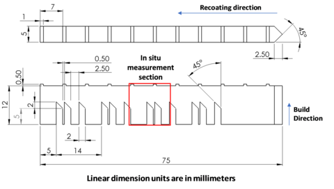
2.1.2 Part geometry: Figure 2 presents a schematic of the part that is 75 mm long, 12 mm tall, and 5 mm wide with 7 mm tall ‘legs’ that form into 45° overhangs below a solid structure. For both AMMT and CBM tests, recoating direction starts at the pointed end with the 45° taper, and proceeds left. A stereolithography (STL) file for the individual part can be found here.
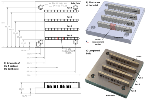
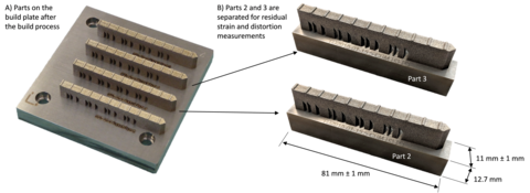
2.1.3 Part layout on the build plate: Four parts are fabricated on each build plate, as shown in Figure 3. Each part is identical. They are spaced by 20 mm along the Y-axis, and they are offset from each other along the X-axis by 0.5 mm so that the recoater blade progressively engages each one. Parts are fabricated in the order they are labeled (Part 1 first, Part 4 last). A STL file of the build plate and 4 parts can be found here.
2.1.4 Feedstock Material: All IN625 and 15-5 powders were obtained from the same respective lots, and kept sealed in original shipment containers until use. Virgin powder was used in each build. Mill Test Certifications supplied by the manufacturer for the IN625 and 15-5 are available.
| IN625 | 15-5 | |
Particle size distribution (PSD)
| D10 = 16.4 μm D50 = 30.6 μm D90 = 47.5 μm | D10 = 20.4 μm D50 = 34.0 μm D90 =50.6 μm |
Chemical Composition
| C = 0.02 % S = <.005 % N = 0.012 % Mo = 8.82 % Nb = 3.97 % Co = 0.17 % Fe = 0.81 % Ti = 0.39 % Mn = 0.04 % Cr = 20.61 % Si = 0.18 % P = <010 % Al = 0.3 % Ni = 64.66 % | Fe = 75.91 % C = 0.02 % Cr = 14.9 % Cu = 3.9 % Mn= 0.1 % Mo < 0.1 N= 0.04 % Nb = 0.3 % Ni = 4.3 % O = 0.03 % P = < 0.01 % S = < 0.01 % Si = 0.5 % |
2.2 Scan Strategy and Parameters
The following presents the scan strategy and scan parameters used by the CBM. The scan strategy and parameters are used for builds in each material (IN625 and stainless steel 15-5). The build parameters and scan strategies are replicated as closely as possible by the AMMT. The slight differences between each machine will be described. The scan strategies for both IN625 and 15-5 steel are identical, including the laser power and speed settings. The only differences in the processing conditions are the recoater blade, which will be discussed in Section 2.2.5, and the power distribution function of the two lasers.
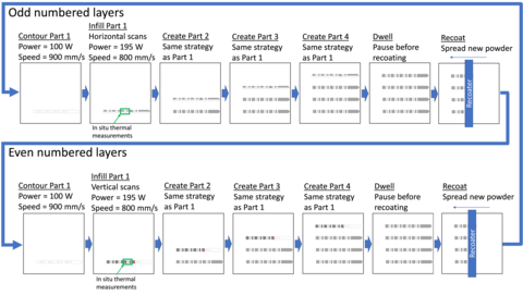
Each layer consists of a contour scan followed by an infill scan. Within each layer, the contour and infill of a part is completed before the next part begins. During odd numbered layers the infill pattern consists of horizontal scans (parallel to the X-axis) that are separated by 0.1 mm (hatch spacing). During even numbered layers, the infill pattern consists of vertical scans (parallel to the Y-axis) that are also separated by 0.1 mm. In between each layer, the build platform is lowered by 0.02 mm so that a new layer of virgin powder can be spread across the powder bed. This process is outlined in Figure 4. the odd and even layers are demonstrated in two different MPEG-4 videos. One is a video that illustrates the scan strategy while the other video is a recording made during several layers from inside the build chamber. The following sections provide more detail of each step. The following information for the CBM is obtained by recording the laser-on/off signal at a rate of 200 MHz and comparing the signal with low-speed and high-speed videos of the process.
2.2.1 Contour of the part features: The contour of each feature on the part is scanned first using a programmed laser power of 100 W and a scan speed of 900 mm/s. The number of contour scans and their timing depend on which features are being created. For instance, as the 12 legs and the base of the part are being scanned in layers 1-250 (Z=0.02 mm to Z=5.00 mm), the laser-on times for legs of similar sizes are consistent. However, since the order of the contouring operations and the starting location of each contour varies from layer-to-layer, the time between legs varies slightly depending on where the laser need to travel to next to melt the next line of material. Furthermore, as the overhang structure begins to form from layers 251-350 (Z=5.02 mm to Z=7.00 mm), the perimeter of the legs and base increase, necessitating a greater amount of time to fabricate these 13 features. However, once the overhang features are complete, the individual leg sections merge, and only the bridge is being fabricated in layers 351-600 (Z=7.02 mm to Z=12.00 mm); only a single contour is required that takes less time than the 13 individual contours. This information is shown in Table 1. Other than some variations between layers due to the contour scan sequence, there is no difference between the contour strategies of the even and odd layers.
Table 1 - Summary of the contouring scan timing for each part in the CBM. The timing is the same for both materials.
| L1, L4, L7, L10 | L2, L5, L8, L11 | L3, L6, L9, L12 | Base | Bridge | |
| Layers 1-250 Laser-on duration (s) | 0.0224 | 0.0124 | 0.0168 | 0.0503 | N/A |
| Layers 251-350 Laser-on duration (s) | 0.0224 – 0.02667 | 0.0124 – 0.01667 | 0.0168 – 0.02111 | 0.0503 – 0.0547 | N/A |
| Layers 351-600 Laser-on duration (s) | N/A | N/A | N/A | N/A | 0.1125 |
In between each contour scan the duration of the laser-off time ranges from 0.0155 s to 0.0255 s, depending on where the previous contour concludes and the next one begins. Once the contours of a single part are complete, the duration of the laser-off time is 0.307 s to 0.363 s before the laser turns back on to begin the first infill scan of the same part.
2.2.2 Infill of the odd numbered layers: All odd numbered layers are processed by the laser traveling at a programmed speed of 800 mm/s using a programmed power of 195 W. It rasters in the horizontal (parallel to the X-axis) direction. The first infill scan line begins at the upper left corner of the part and scans to the right (+X). During the fabrication of the legs, the laser scans from one feature to the next along a constant Y coordinate until it reaches the end of the furthest feature to the right, at which point the laser turns off as the scan direction reverses. This process is illustrated in Figure 5. The laser-on time for each feature depends on the width of the feature along the current scan trajectory. The duration that the laser is off between features depends on the length of the previous feature (if the Y coordinate does not change). The laser-off time is presented in Figure 5 and in Table 2, which also reports the laser-on time for each feature.
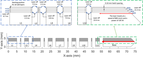
Table 2 - Laser-on/off times of the CBM during the processing of different features during the odd numbered layers. This is the same for both materials.
| Laser-ON time of the CBM for each feature | ||||||
| L1 | L4, L7, L10 | L2, L5, L8, L11 | L3, L6, L9, L12 | Base | Bridge | |
| Layers 1-250 Laser-on duration (s) | 0.0062 | 0.0062 | 0.0006 | 0.0031 | 0.0208 – 0.0238 | N/A |
| Layers 251-350 Laser-on duration (s) | 0.0062 | 0.0062 – 0.0087 | 0.0006 – 0.0031 | 0.0031 – 0.0056 | 0.0208 – 0.0263 | N/A |
| Layers 351-600 Laser-on duration (s) | N/A | N/A | N/A | N/A | N/A | 0.0906 – 0.0938 |
| Laser-OFF time of the CBM after each feature | ||||||
| Turn around on left-side | L1, L4, L7, L10 | L2, L5, L8, L11 | L3, L6, L9, L12 | Base | Turn-around on right-side | |
| Layers 1-250 Laser-off duration (s) | 0.0067 | 0.0079 | 0.0023 | 0.0480 | 0.0253 | 0.0213 |
| Layers 251-350 Laser-off duration (s) | 0.0067 | ≤ 0.0079 | ≤ 0.0022 | ≤ 0.0480 | ≤ 0.0253 | 0.0213 |
| Layers 351-600 Laser-off duration (s) | 0.0067 | N/A | N/A | N/A | N/A | 0.0213 |
2.2.3 Infill of the even numbered layers: All even numbered layers are processed by the laser traveling at a programmed speed of 800 mm/s and using a programmed power of 195 W. It rasters in the vertical (parallel to the Y-axis) direction. The first infill scan line begins at the lower left corner of the part and scans upward (+Y). During these layers, the infill of each feature is completed before the laser begins melting material in the next. The direction of each scan alternates regardless of whether the laser is continuing to scan a single feature or is transitioning between features. The laser-on times and laser-off times are consistent within features (excluding the right edge that forms a point). However, the laser-off duration is longer between features. This information is presented in Figure 6 and Table 3.
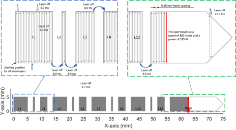
Table 3 - Laser-on/off times of the CBM during the processing of different features during the even numbered layers. This is the same for both materials.
| Laser-on time of the CBM for each feature | ||||
| Within a leg | Base / Bridge consistent width | Base / Bridge pointed end | ||
| Layers 1-250 Laser-on duration (s) | 0.0062 | 0.0062 | 0.0001 – 0.0062 | |
| Laser-off time of the CBM for each feature | ||||
| Within a leg | Between features | Base / Bridge consistent width | Base / Bridge pointed end | |
| Layers 1-600 Laser-off duration (s) | 0.0067 | 0.0080 | 0.0067 | 0.0008 – 0.0067 |
2.2.4 Time between parts within a build: Within a layer, the time between the completion of the last infill scan line on a part and the beginning of the first contour of the next part ranges from 0.307 s to 0.363 s. This time variation is a function of where the last infill scan concludes and where the first contour scan begins. The contours are performed in a different order with a different starting position in each layer, thus causing the variation in time between parts.
2.2.5 Total layer time and recoating: During the fabrication of the legs (Z=0.02 mm to Z=5.00 mm), the average layer time is 52 s. That is, 52 s pass from the time the first contour begins on layer n to the time the first contour begins on layer n+1. Considering it takes on average 26 seconds to complete the layer for all 4 parts, a significant amount of time is spent before the laser begins melting material for the next layer. The recoating time in the CBM is shorter than in the AMMT, so a dwell is imposed in the CBM to make the average layering time approximately equal.
Recoating is performed using a solid recoating blade. When processing 15-5 stainless steel, a ceramic recoating blade is used. When processing IN625, the blade is high-strength steel. The recoating blade spreads powder across the powder bed surface at a speed of 80 mm/s.
2.2.6 Summary of the scan parameters: Table 4 presents a simplified summary of the scan strategy and parameters. Where appropriate, differences between the CBM and AMMT are highlighted.
Table 4 - Summary of the build parameters for both the CBM and the AMMT. The same parameters are used to process each material.
| Parameter and description | CBM | AMMT |
| Total number of layers | 625 | 625 |
Layer height
| 20 μm | 20 μm |
| Contour Scan speed | 900 mm/s | 900 mm/s |
| Contour Laser power | 100 W | 100 W |
| Infill Scan Speed | 800 mm/s | 800 mm/s |
| Infill Laser Power | 195 W | 195 W |
Hatch Distance
| 100 μm | 100 μm |
Time between infill scan lines
| 6.70 ms | 3.03 ms |
Laser spot size (FWHM)
| 50 μm (estimated) | 45.0 μm |
| Inert gas | Nitrogen | Argon |
Oxygen level
| ≈ 0.5% | < 0.08% |
3. Description of Benchmark Comparisons
Several post-process measurements are performed to facilitate a series of benchmark challenges, including residual strain measurements, distortion resulting from partial removal from the build plate, and microstructural characterization. Before these measurements can be performed, the 4 parts on each build plate are separated from one another via EDM cutting, as shown in Figure 7. As a result, the parts used for distortion and residual strain measurements (Parts 2 and 3) are attached to a smaller portion of build plate material than during the build. The remaining build plate material measures 81 mm ± 1 mm long, 11 mm ± 1 mm wide, and (12.7) mm thick.
3.1 Part Deflection: Benchmark Challenge CHAL-AMB2018-01-PD
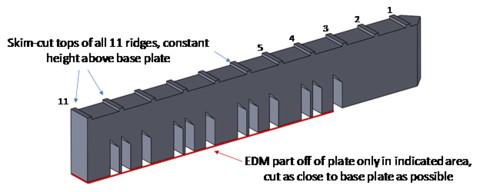
After being built, the parts remain on the build plate. The tops of the 11 ridges are skim cut to remove the rough as-built surface. The vertical height, relative to the base plate, of the top of both side edges of each ridge is measured. Next, the part is EDM cut such that only the end portion of the part remains attached to the plate (see figure), and the cut section of the part will deflect upward from relaxation of the as-built residual stresses.
For these benchmark comparisons, the part distortion is defined by the vertical deflections of all measured ridge edges. Thus, δi = ziafter - zibefore, where δi is the vertical deflection of edge i.
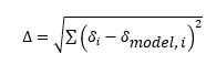
Distortion Results Comparison: The δi will be measured at all 22 points (at approximately the center of the edge of each ridge on the top surface, both sides of each ridge measured), and modelers should attempt to extract similar information from their models. After the benchmark measurement data are released, modelers should compare the difference between each measured and modeled distortion point. Modelers may also calculate a cumulative distortion value, being the root sum-square-error between the measured and modeled values:
3.2 Residual Elastic Strain: Benchmark Challenge CHAL-AMB2018-01-RS
Residual elastic strain (RS) within the as-built IN625 and 15-5 steel parts is measured using neutron diffraction on the BT8 diffractometer at the NIST Center for Neutron Research (NCNR).Some supplementary RS measurements will be conducted at the Cornell High Energy Synchrotron Source (CHESS) and the Los Alamos Neutron Science Center (LANSCE). These supplementary measurements will not be available for the May 18, 2018 data release, but will be added to the AMB2018-01 data archive later.
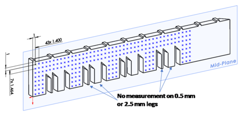
Figure 9 shows the locations where NCNR measurements are being conducted.Lattice strains along X, Y, and Z directions will be measured at each location.It is important to note that all NCNR measurements will be conducted using approximately cubic sample volumes, 1.5 mm on an edge, centered on the midplane of the specimen.
Residual Strain Results Comparison: Modelers should extract axial residual strain values (exx, eyy, ezz) located on the section plane shown in Figure 9, and based on the coordinate system shown. Modelers should compare, side-by-side, color map or contour map images of each of the three axial strain fields.
3.3 Microstructure
Microstructure studies are conducted on thick (nominal 5 mm) and thin (nominal 0.5 mm) legs of the as-built specimens to evaluate the sensitivity of the microstructure evolution to the local geometry and thermal conditions of the build. Specific legs are numbered as shown below. Measurements include 1) optical microscopy at NIST and/or NRL, 2) scanning electron microscopy (SEM) measurements at NIST, including secondary electron (SE) imaging, electron backscatter diffraction (EBSD), and energy dispersive spectroscopy (EDS), 3) synchrotron X-ray powder diffraction at beamline 11BM at the Advanced Photon Source (APS), Argonne National Laboratory (ANL), and 4) ultra-small-angle X-ray scattering (USAXS) and associated techniques at beamline 9ID-C at the APS. In addition, a more limited set of measurements are conducted on samples that have undergone a RS relief to evaluate the sensitivity of the as-built microstructure to these isothermal heat treatments. The RS relief heat treatments are 1 h at 650 °C for 15-5 steel, and 1 h at 800 °C for IN625. The USAXS measurements are conducted in situ during these RS relief heat treatments, with a time resolution of approximately 6 min.
Samples are cut along transverse (y-z plane) and longitudinal (x-y plane, parallel to the base plate) orientations. Thin transverse specimens are used for all powder diffraction and USAXS measurements; SEM specimens are both transverse and longitudinal.
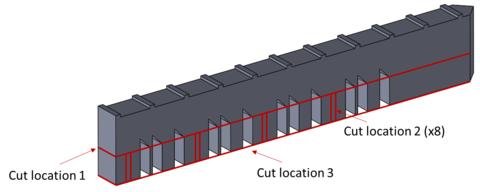
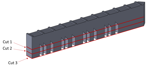
The thin transverse specimens are cut from the bridge structure as follows. First, the top of the bridge is cut off using EDM as shown in Figure 11. Second, the 8 vertical cuts are made. These cuts produce four 0.5 mm thick specimens, from the centers of the 5 mm thick legs (as shown above), and parallel to the Y-Z plane. Finally, the legs are cut from the base plate using a single EDM cut labeled cut location 3 in the figure.
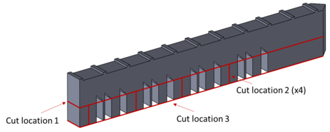
The transverse SEM specimens are cut from the bridge structure as follows. First, the top of the bridge is cut off using EDM as shown above. Second, the 4 vertical cuts are made. These cuts produce two mirrored specimens for each leg. Finally, these pieces are cut from the base plate using a single EDM cut as shown in the figure above.
The longitudinal SEM specimens are cut from the bridge structure as follows. First, the top of the bridge is cut off using EDM as shown above. Second, the legs are cut in half parallel to the base plate. Third, the lower half of the legs are cut from the base plate.
3.3.1 Optical Microscopy: Transverse and longitudinal specimens from polished surfaces of the thick and thin legs are examined using standard optical microscopy techniques. Measurements from these images provide information on the amount, morphology, and distribution of porosity.
3.3.2 SEM: Transverse and longitudinal specimens from thick and thin legs are examined using all of the SEM measurement methods described above. Both polished and chemically etched samples are examined as needed. These measurements provide information on the primary phases, grain size, aspect ratio, local crystallographic orientations, dendritic/cellular microstructure, and elemental segregation.
- Benchmark Challenge CHAL-AMB2018-01-MS: predict any/all of the following – primary phases, grain size, aspect ratio, dendritic vs cellular microstructure, primary arm spacing, and elemental segregation within the thick and thin legs, as observed on transverse and longitudinal views as described above. Regarding phase predictions, part of this aspect of the challenge includes being able to make assumptions about what phases might be present.
3.3.3 Powder XRD: These transmission measurements use thin transverse specimens cut from 5 mm and 0.5 mm thick legs as shown above. Conventional metallographic polishing methods are used to thin these specimens to an approximate thickness of 100 μm. Powder X-ray diffraction measurements are conducted at the APS and subsequent analysis identifies the phases and phase fractions within the specimens, including the most common precipitates. Details concerning the powder diffraction instrument may be found here. As-built IN625 is almost entirely single phase, but martensitic stainless steels are more complex.
- Benchmark Challenge CHAL-AMB2018-01-PF: predict the phases and phase fractions within the transverse samples from the thick and thin legs of the as-built 15-5 specimens.
3.3.4 USAXS: With a time resolution of about six minutes, the USAXS instrument at the APS uses small angle scattering to obtain information about a sample’s microstructure over a size range from micrometers to below one nanometer, while simultaneously using diffraction to probe the phases present. The instrument uses ultra-small-angle X-ray scattering (USAXS) to study the larger length scales, pin-hole small-angle X-ray scattering (SAXS) to study the smaller length scales, and wide-angle scattering (X-ray diffraction) to obtain the phase information, including the most common precipitates. Detailed information on this unique instrument and its use may be found here. These transmission measurements use thin transverse specimens cut from 5 mm and 0.5 mm thick legs as shown above. Conventional metallographic polishing methods are used to thin these specimens to an approximate thickness of 35 μm.
- Benchmark Challenge CHAL-AMB2018-01-PFRS: Phases and phase fractions as function of time for RS anneals of IN625 and 15-5, from transverse specimens cut from thick and thin legs as described above.
4. Description and Links to Associated Data.
The following data will be provided on February 20th to assist in the development of models and simulations. Benchmark measurement results data will be provided on May 19th. Each link directs the user to a downloadable zip folder, which contains the data briefly described below, as well as a document with thorough description of the zip folder contents, file structures, and information pertaining to how the data or measurements were generated or obtained.
The following data files are available facilitate model development:
- STL file of the individual bridge structure
- STL file of the build plate and 4 parts
- MPEG-4 video illustrating the scan strategy used to fabricate one of the bridge structures
- MPEG-4 video showing several layers of the build acquired from inside the CBM build chamber
- Manufacturer supplied Mill Test Certificate for the IN625 powder
- Manufacturer supplied Mill Test Certificate for the 15-5 powder
Disclaimer
The National Institute of Standards and Technology (NIST) uses its best efforts to deliver a high-quality copy of the Database and to verify that the data contained therein have been selected on the basis of sound scientific judgment. However, NIST makes no warranties to that effect, and NIST shall not be liable for any damage that may result from errors or omissions in the Database.
Certain commercial entities, equipment, or materials may be identified in this document to describe an experimental procedure or concept adequately. Such identification is not intended to imply recommendation or endorsement by the National Institute of Standards and Technology (NIST), nor is it intended to imply that the entities, materials, or equipment are necessarily the best available for the purpose.
Contacts
-
(301) 975-6032
-
(301) 975-2265