Reflpak

Reflpak provides support for data reduction and simple fitting of ncnr data. Reduction is driven by reflred, which allows you to view raw X-Ray, NG-1 and NG-7 data files and reduce them to a reflectivity curve. For simple analysis there is the layer-based reflfit and reflpol programs. Limited help is available within the programs via the F1 key or online (reflred help and reflfit/reflpol help). Support for linux and OS/X were available in much older versions. Source is available on github.

To run reflred, you will need to download Octave from the link above and install it. Before starting reflred, start Octave, and type the following at the command prompt:

    listen(1515,'nofork')

This sets up the octave server to provide computational support for the reduction program.

Citing reflfit, reflpol, reflred

Acknowledging use of reflpak in publications may be done by making a reference to this site. For example:

The programs from the reflpak suite were used for elements of the data reduction and analysis.[1]

[1] P.A. Kienzle, K.V. O'Donovan, J.F. Ankner, N.F. Berk, C.F. Majkrzak; http://www.ncnr.nist.gov/reflpak. 2000-2006

reflred

Many raw data files are required to produce one reflectivity curve. Individual runs are used to cover different parts of the Q range due to things such as differing counting times, sampling densities or beam attenuation. With polarized beam, the data for each polarization state (A, B, C or D) is taken separately. In an extreme case (polarized data with positive and negative Q ranges each split into several runs) over 100 files may be required to produce a single reflectivity curve.

The attenuators are placed in the beam by hand, so each time an attenuator is changed, there will be another file created. Because the detector needs time to recover between events, we need attenuators whenever the rate of neutrons entering the detector is too high. This is mainly an issue for slit scans because then the detector is exposed directly to the beam.

The motor control program only allows motors to be moved by fixed increments during a single run. At low angles the user has fixed slits, so low angle data must be in a separate run. Depending on what you are measuring, you will want to sample some parts of the reflectivity curve more densely than others. Each change in sampling density requires a new run.

The measurable reflectivity signal can change by seven orders of magnitude from below the critical angle where it is one, to high angles where it is indistinguishable from background. To get statistically significant counts throughout the entire range, different sections are measured for different times. Whenever the measurement time changes, a new run is needed.

One instrument (NG-1) has polarizers and spin flippers to change the polarization state of the neutrons. A complete set of data consists of A,B,C,D files depending on which of the pair of flippers is activated. Sometimes reflectivity is measured through front and back surfaces, so each positive Q run will have a corresponding negative Q run.

For a variety of reasons the same Q range is often measured several times. Sometimes it is because the sample is dynamic. You will reject the first few passes because the specular curve is still changing, but you will want to combine the remaining passes in the final reflectivity. Plus there are the usual problems that crop up during an experiment which cause some runs to be aborted or some ranges to be remeasured.

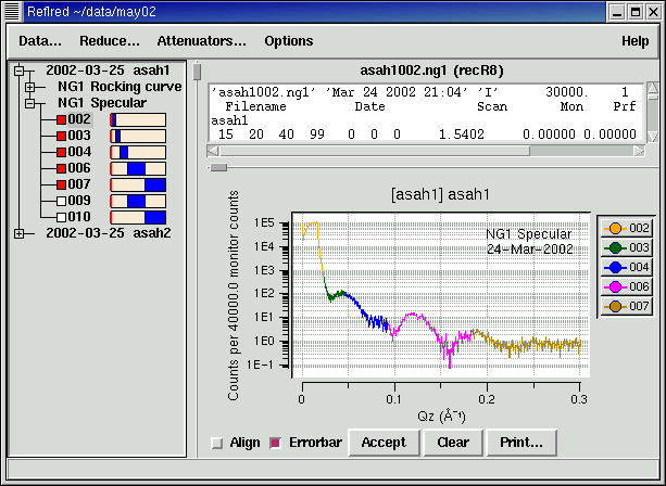Data selection screen. Runs are categorized by curve type, and displayed with range of data in the run (blue bars in file list). Selected runs are displayed on the graph in different colors. The raw data file for one run is displayed.

To make sorting through the data easier, our software automatically categorizes each file according to what it is trying to measure. This is easy for reflectometry because that information is completely determined by the motor movements as recorded in the data file. The data range is displayed along with the run number. This makes it easy to see which runs compose the entire Q-range of the curve without having to select the files or read from the log book. Double-clicking the first file in the Q-range automatically selects all files of the same type which extend the Q-range. Data taken with different flippers or different slits or at different temperature or different field are skipped. You can add or remove files individually, and with a little extra effort you can force otherwise incompatible files to be selected together. An ongoing theme is to provide convenience without sacrificing flexibility.

Even as a tool for sorting data files without performing any reduction, experienced users have found our software to be worthwhile. Being special purpose software it knows how to plot reflectometry data and automatically normalize for things like monitor count. What you can do with a double click would take several minutes to do with command line tools. The result is that data reduction which used to take hours can now be done in minutes.

Even better, our software encourages you to examine the data at each step of the reduction process. In one case a subtle problem with the instrument controller lead to a small discrepency in one of the scans. Because the data is visible at every step of the way the discrepency was easy to spot. With command line and batch files, there isn't a strong inclination to view the data every step of the way, and the discrepency wasn't noticed.

For new users the software is a boon. Yes you benefit as much from the data browsing capabilities as the experienced users, but you also benefit from the consistency checks which restrict the data that can be selected together. Furthermore certain questionable data points such as those in which the data rate exceeds the known recovery time for the detector are automatically tagged for exclusion. While it may not be obvious to why the points are being excluded, it should be enough of a clue that you will ask a more experienced user what is going on. Better that than to quietly accept questionable data. You can override the exclusion easily enough in keeping with the theme of convenience and correctness without sacrificing flexibility.

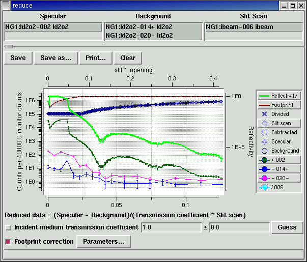Data reduction screen.

Once the files are selected the data reduction process is fairly straight forward. A set of specular, background and slit scans are selected. Specular runs are averaged and the average background is subtracted. The result is divided by the slit scan and by the incident medium transmission coefficient if the beam is attenuated by the sample environment. If the data was taken with fixed slits at low Q, you need to apply a footprint correction to account for the fact that some of the beam spills over the edges of the sample.

There are of course complications. For example, the slit scan is based on slit configuration rather than angle so specular and background data need to carry slit information along with them so they can be normalized later on. That means the data saved in intermediate files must also record the slits associated with each data point. This complicates saving and reloading data files. There are also the same sorts of complications which arise with data selection: the software tries to ensure that the scans selected for reduction are consistent, allowing the user to override if necessary.

Again the GUI interface allows you to easily learn the necessary steps for data reduction. The software can keep track of the state of the data reduction and warn if for example you try to do a footprint correction before selecting the slit scan which will normalize the data [this is work in progress].

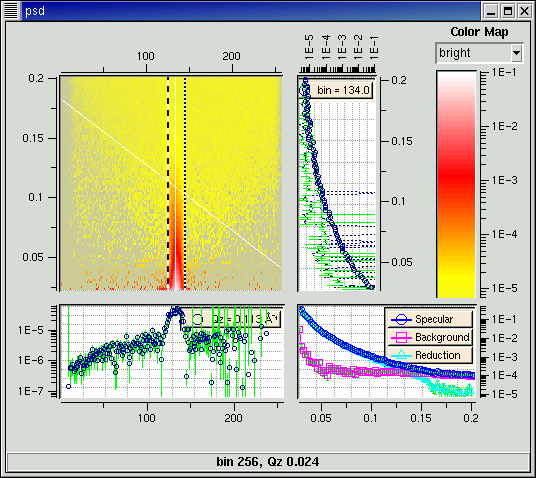Position sensitive detector

One instrument (NG-7) has a position sensitive detector available. With this detector, each row of the datafile effectively measures a rocking curve. Integrating over the peak of this curve gives the specular reflection for that Q, with the surrounding bins giving the background you need to subtract. For PSD data, you can select the range over which you are going to integrate. Since NG-7 records a monitor count which can be divided out of the measured signal without the need of a slit scan, the curve recovered from the PSD is already shows reduced reflectivity.

Online help is available within the program.

Reflfit and Reflpol

Reflfit and its polarized neutron sister reflpol are two of our reflectometery analysis program. They let you fit your reduced reflectivity data to a layer model.

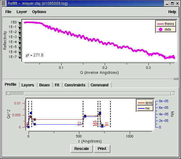
You can directly manipulate the layer profile by dragging the depths and control points around the graph.

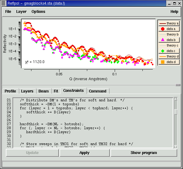
You can encode arbitrary constraints among the parameters.

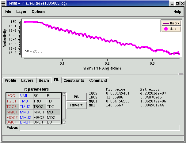
You can fit to any of the layer parameters using a Levenburg-Marquardt non-linear fitting algorithm. You can also fit to artificial parameters which encode the constraints, such as the total depth of a set of equally thick layers.

Online help is available within the program.