Sequential Bayesian Experiment Design

Summary

Every day, across the globe, people measure things.  Many measurements are direct: weight from a scale, volume from a measuring cup, length from a tape measure.  But often, the things we want to measure (estimate, really) are parameters in a model.  The slope and intercept of a line, an exponential decay rate, and a peak’s position, amplitude, and width are common examples.  For parameter estimation, it is common practice to make a series of measurements and then find the parameter values that best fit the theoretical curve to the data.  For a more efficient alternative to this measure-then-fit strategy, we create and publish software that implements sequential Bayesian experiment design, a statistical method that interprets measurement data “on-the-fly” and adaptively guides measurements toward the most useful settings, ultimately conserving measurement resources and/or improving measurement uncertainty. This feature is very helpful in situations where the measurements are expensive relative to computational costs.

Description

We develop and publish the optbayesexpt python package. The package implements sequential Bayesian experiment design to control laboratory experiments for efficient measurements. The package is designed for measurements with:

• an experiment (possibly computational) 
• that yields measurements and uncertainty estimates, 
• and that can be controlled on the fly by one or more experimental settings, and with
• a parametric model, i.e., an equation that relates unknown parameters and experimental settings to measurement predictions.  

The OBED method represents the unknown parameters random variables with a probability distribution. Measurement data typically narrows the parameter distribution, i.e., narrow distributions correspond to small uncertainties.  Using the parameter probability distribution, the algorithms do two tasks. In a learning step, the algorithm uses Bayesian inference to incorporate new measurement data and to refine the probability distribution.  In this way, the algorithm maintains up-to-date “knowledge” of the parameters based on all accumulated data.   Then, in an advising step, the algorithm uses likely parameter values to determine experimental settings that have the best chance of refining the parameter distribution.  This calculation permits a strategy that avoids wasting resources on measurements that are unlikely to improve results.

The optbayesexpt python package simplifies development of efficient laboratory measurements. To accommodate instrument control programs written in other languages, optbayesexpt includes a server script that runs in the background to provide Bayesian inference and measurement settings via TCP messages.

The optbayesexpt theory, software documentation and example descriptions are available at https://pages.nist.gov/optbayesexpt.  The python package and example scripts can be downloaded from https://github.com/usnistgov/optbayesexpt.

Examples

Measuring a resonance

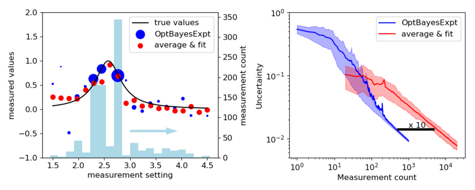
Determining the center of a peak is a task that is common across many branches of science and engineering.  In this example, we compare simulated measurements using measure-then-fit (least squares) with OBED strategies.  The right panel shows results after 1000 individual measurements, each with signal/noise = 1.  Red circles show averages of 50 values at each of 20 settings.  The blue circles are also average values with the number of values at each setting shown by the histogram.  Circle areas are proportional to the resulting weights of the points, 1/σ2.  To best determine the peak center, the OBED algorithm focuses measurements on the sides of the peak.

The right panel traces how uncertainty decreases as data accumulates comparing measure-then-fit and OBED methods.  Solid lines are mean values of uncertainty from 100 runs of 20 000 measure-then-fit and 1000 OBED measurements.  The region between the 20th and 80th percentile is shaded.  Least squares fits that did not converge were thrown out, biasing the red curve downward for low measurement counts.  Both methods converge to a 1/√N behavior, but the OBED algorithms produced a 10X decrease in measurements needed to attain comparable uncertainty.

 

Comparison of uniform scans, averaged and fit with OBED methods

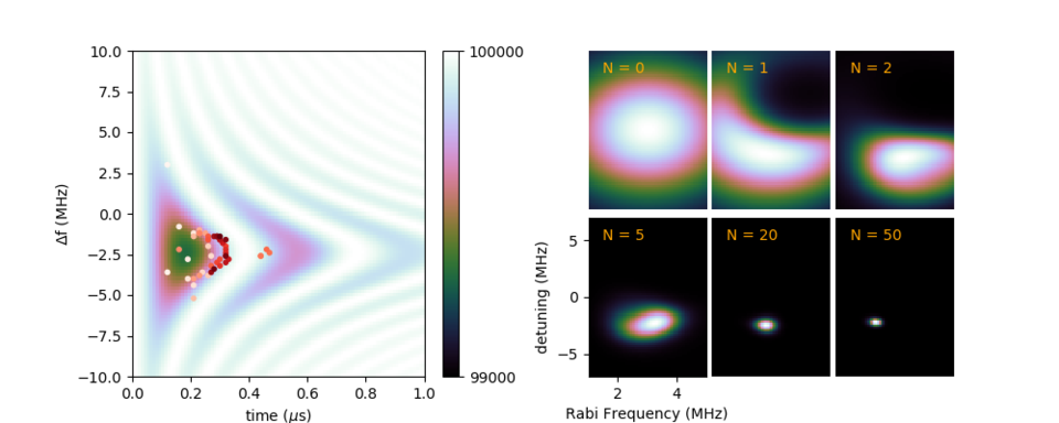
Tuning for quantum control

Quantum technology relies on the ability to reliably manipulate qbit states.  For example, radio- or microwave-frequency pulses can be used to change a spin state from |up> to |down>, and patients benefit from MRI scans that use these methods.  In fact, many systems exhibit similar behavior, and the general phenomenon is known as Rabi oscillation.  In this example, we have simulated a tuning process to determine the desired frequency and duration of pulses to reliably flip electron spins.  The right panel shows simulated measurement points in order from pink to red over a background of the model “true” mean photon count.  Simulated measurements include Gaussian noise (σ = 300, approximately the same size as the overall contrast).  The right panels shows the flip-rate / rf-frequency probability distribution evolving with the number (N) of measurements.  The color scale is stretched in each case.

 

Measurements of transition probability vs. pulse length and detuning