Summary
The long records (sometimes over 100 years) of surface temperatures available from meteorological monitoring stations in the Unites States can be a valuable resource for estimating the magnitude of temperature trends attributable to changes in the climate. Examples of such records may be found at https://www.ncdc.noaa.gov/. However, for some of these records, especially the very longest ones, we find artifacts, unrelated to the underlying climate that affect estimates of the trend. These artifacts are often abrupt changes that occur because for example the location of the monitoring station changes or the instrumentation changes. Other types of non-climate related artifacts like urban heat island effects can be found too.
The purpose of this project is to examine statistical approaches to detecting these artifacts directly from the records, i.e., ignoring meta-data like dates of location changes that might be available. This is important for two reasons. First, the total number of stations is very large, making human examination of all records onerous. Second, and more importantly, we are not guaranteed that all of the salient events were recorded. To date, three general statistical approaches have been examined, control charting, non-parametric smoothing, and a fully parametric change point model with estimation by Bayesian inference.
This project is a part of the Greenhouse Gas Measurements Program at NIST.
Description
DESCRIPTION:
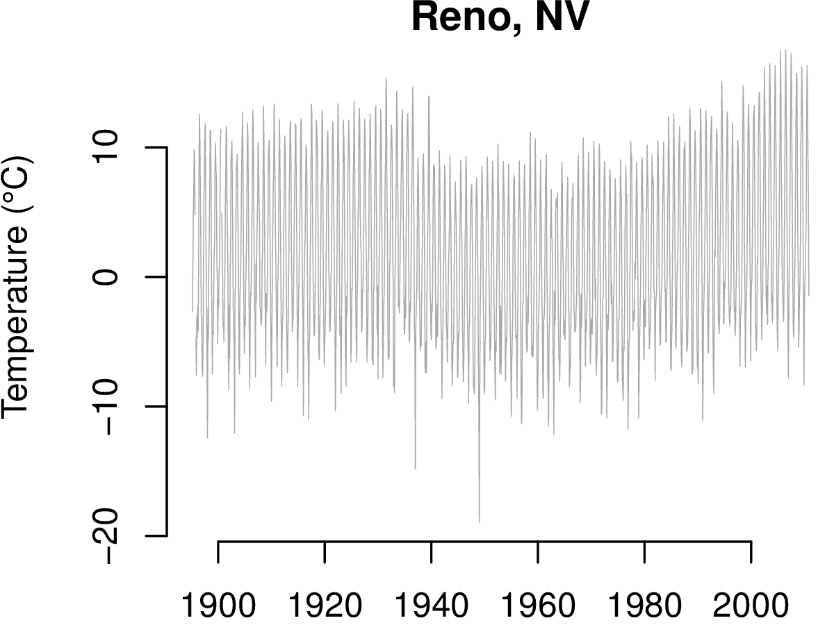
For the purpose of exposition, consider the record daily minimums averaged by month for a station near Reno Nevada.

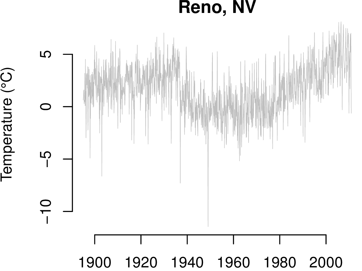
There is a clear drop in the level between 1920 and 1940 and a positive drift starting at about 1980. There is also however, considerable variability due to seasonal changes that can mask more subtle artifacts. The seasonal effects are removed using the methods of Cleveland et al. (1990). Here is the result.

The level change and drift are more striking after removing seasonal effects, and these are the data subjected to the change point detection methods.
Control Charting
Control charting is a statistical technique that is often used to detect changes in a manufacturing processes, e.g., to detect if too much or too little cereal is being put into the bags on a production line. Based on in-control data, control limits are set, and if an observation falls outside of the limits, an alarm is triggered. Since control charts are designed for detecting level shifts and drifts they represent a natural choice for our problem. The method of Zhang (1998) is also a natural fit because it allows for autocorrelation (as opposed to statistically independent data), a very important allowance for temperature data. The most difficult problem to overcome with control charting is ensuring that the control limits have been created using a part of the series that is in-control.
Smoothing
Another approach is to smooth the noisy data with a non-parametric smoothing procedure like adaptive weights smoothing (Katkovnik et al., 2006), which was developed for image processing and is especially sensitive to edges (level shifts). The first differences of the smooth curve may be used to asses the plausibility of a change from one time to the next. A Monte Carlo algorithm may be used to set the magnitude of a difference that indicates a change. This approach does not suffer from the need to construct limits based on in-control data like the control charting method, but it is unlikely to detect drifts because of the first differencing.
Parametric Model
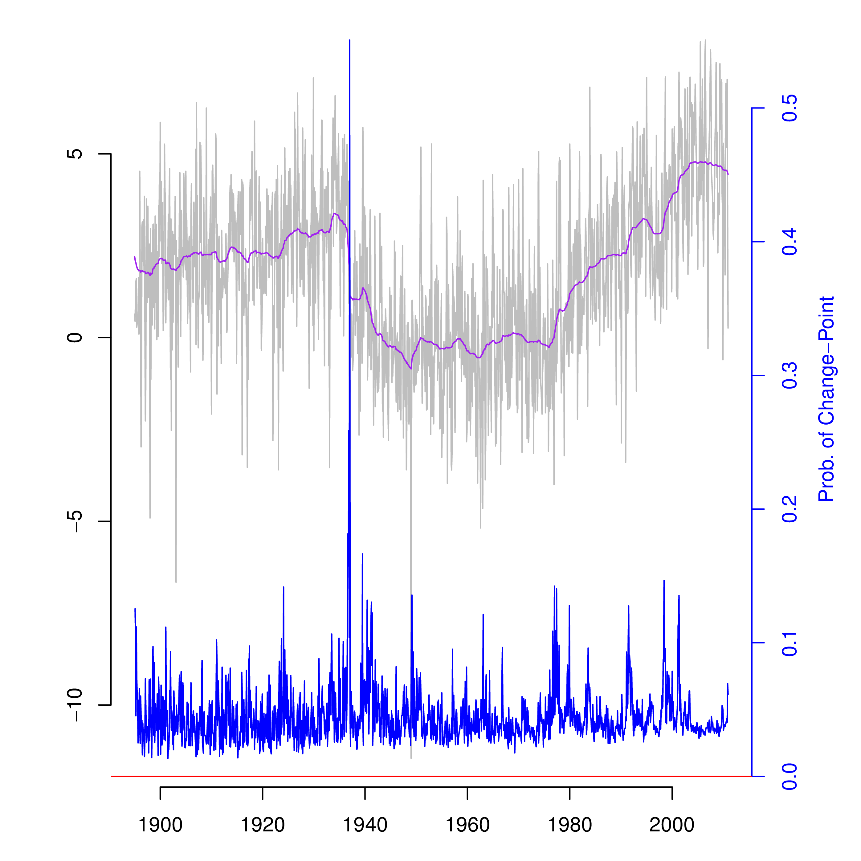
The parametric modeling approach takes the autocorrelation structure of the data to follow that of a stationary autoregressive process, and it also allows for the possibility of a different mean level at each point in time. Associated with each mean level is a parameter for the probability that this mean level differs from the previous one. The model is described in detail by McCulloch and Tsay (1993). Since there are more parameters than observations (over twice as many) it is necessary to take a Bayesian approach to inference using informative priors. This makes the automation of the algorithm more difficult than for control charting and smoothing because user tuning of the prior distributions may be necessary. Here are the results of applying this algorithm to the Reno data which imply that with proper tuning it is possible to detect both level shifts and drifts without the need for assuming a part of the series to be in-control.

For completeness, note that the large level shift between 1920 and 1940 was due to changing the location of the station, and the positive drift starting about 1980 is a heat island effect. Also note the small—but noticeable—dip around the year 2000. This was due to moving the station from one end of the runway to the other and then back at the Reno airport.
Future Directions
While the fully parametric approach is very promising, improvements are possible. A robust, data set specific way to automatically specify prior distributions and the nature of the autocorrelation (the order of the autoregressive process) is necessary for full automation. Moreover, a mechanism for deciding if a change actually occurred at time t is also imperative. The mechanism should balance the risk between false positives and negatives as well as allow the user input about the relative importance of making each type of error. Lastly, the required computation is onerous. The above results took more than an hour to produce. A strategy to reduce computation time is also important.
References
R. B. Cleveland, W. S. Cleveland, J.E. McRae, and I. Terpenning (1990) STL: A Seasonal-Trend Decomposition Procedure Based on Loess. Journal of Official Statistics, 6, 3 – 73.
N. F. Zhang (1998) A Statistical Control Chart for Stationary Process Data. Technometrics, 40, 24 – 38.
V. Katkovnik, K. Egiazarian, and J. Astola (2006) Local Approximation Techniques in Signal and Image Processing. SPIE Press Monograph Vol. PM 157
R. E. McCulloch and R. S. Tsay (1993) Bayesian Inference and Prediction for Mean and Variance Shifts in Autoregressive Time Series Journal of the American Statistical Association, 88, 968 – 978.
Major Accomplishments
- (Presentation) 9th International Temperature Symposium held in Los Angeles, CA, March 19 - 23, 2012
- (Publication) A. L. Pintar, A. Possolo, and N. F. Zhang (2013) Statistical Methods for Change-point Detection in Surface Temperature Records in Temperature: Its Measurement and Control in Science and Industry, Volume 8, Proceedings of the Ninth International Temperature Symposium.

