Official websites use .gov
A .gov website belongs to an official government organization in the United States.
Secure .gov websites use HTTPS
A lock (
) or https:// means you’ve safely connected to the .gov website. Share sensitive information only on official, secure websites.
How UTC(NIST) Works
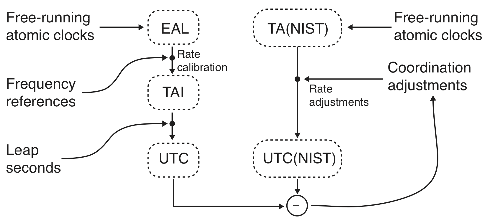
UTC(NIST) works by continuously operating its ensemble of atomic clocks under carefully controlled environmental conditions. The clocks are continuously measured to determine their relative stability, and the measurement data is input to a time scale algorithm, called AT1. The AT1 algorithm then generates a composite oscillator, called TA(NIST), that serves as the primary oscillator for the UTC(NIST) time scale. TA(NIST) has both reliability and performance advantages over any individual clock. For example, it is designed to keep running if any of the individual clocks fail, and it is also designed to be more stable than any of the individual clocks. However, TA(NIST) is not the same thing as UTC(NIST), it is a free-running time scale that is not adjusted. UTC(NIST) is generated by applying coordination adjustments to TA(NIST) so that that UTC(NIST) agrees in time (synchronization) and in frequency (syntonization) with UTC.
This process, shown in Figure 1, is again similar to the way that UTC works. The BIPM utilizes a time scale algorithm called ALGOS that is similar to AT1. ALGOS computes a free-running atomic time scale called EAL, that is similar to TA(NIST). The difference, once again, is that UTC(NIST) produces physical signals, and that UTC does not. The physical signals, in the form of one pulse per second (PPS) signals for time, and 5 MHz signals for frequency are distributed through various distribution amplifiers in the NIST laboratories. A reference plane for the 1 PPS timing signals indicates the point where the signals are exactly “on time”. When necessary, leap seconds are inserted into UTC and into the UTC(NIST) time codes, but do not change the physical UTC(NIST) signals.
The following sections briefly describe the various elements of UTC(NIST), including the atomic clocks, the measurement systems, the ATI time scale algorithm and the free-running TA(NIST) time scale, and the realization and generation of UTC(NIST) as a physical signal.
The Atomic Clocks - More than 20 atomic clocks are measured and tracked at the NIST laboratories in Boulder, Colorado, and as noted earlier, from 10 to 15 atomic clocks are typically included in the time scale ensemble. The number of clocks varies because some clocks are withheld from participating for periods following technical failure or repair, because some contribute only to an independent, redundant time scale, and because some are physically moved when necessary to support other experiments. However, the time scale was designed so that changes in the clock roster, regardless of how often they occur, have minimal impact on the performance of UTC(NIST).
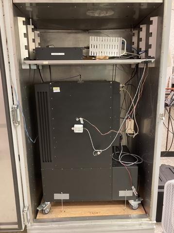
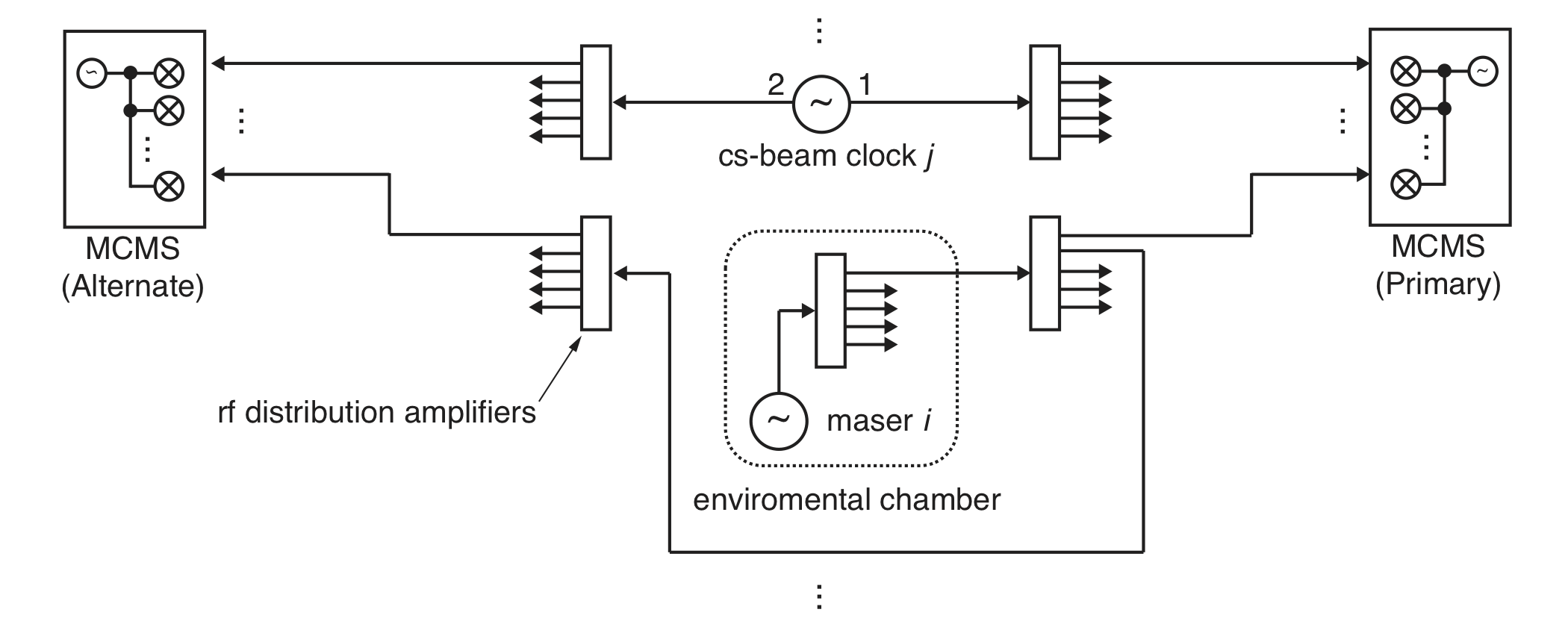
About 2/3 of the atomic clocks that support the UTC(NIST) time scale are hydrogen masers, and about 1/3 are cesium beam clocks. Hydrogen masers benefit from careful environmental control of temperature and humidity and are each installed in independent environmental control chambers, as shown in Figure 2. The cesium beam clocks are also environmentally controlled, although they are less susceptible to environmental fluctuations. Each atomic clock produces a standard frequency output signal in the form of a 5 MHz sine wave. These signals are transported by high-isolation distribution amplifiers and high quality cables before measurement or transmission between laboratories.
The individual clocks in the ensemble are not adjusted, but instead are allowed to free run without adjustment. Their frequency stability is estimated with metrics such as the Allan deviation (ADEV), which is expressed mathematically as \( \sigma_y(\tau) \) and which estimates how much the frequency of the clock will change over a given interval, \( \tau \). A companion metric called the Time deviation (TDEV, expressed mathematically as \( \sigma_x(\tau) \) ) can estimate the time stability, or how much the time will change over a given interval \( \tau \). These stability estimates can help determine the expected holdover performance of a clock between adjustments.
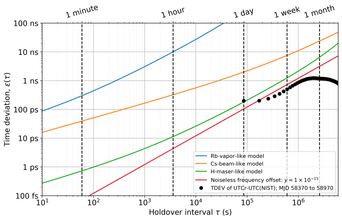
Figure 3 uses time stability estimates to illustrate the holdover performance of several types of atomic clocks, including the cesium beam and hydrogen maser clocks used in the NIST time scale. As shown in the figure, holdover performance of ≤ 10 ns per week requires the use of high-performance cesium-beam clocks. Holdover performance of about 1 ns per week requires the use of a hydrogen maser, as no other commercially-available atomic clock with comparable performance and reliability currently exists.
Figure 3 also shows that over an interval of about one day, the stability of UTCr – UTC(NIST) is at least as good as the stability of a single hydrogen maser. Over longer intervals, UTC(NIST) performs somewhat better than a single maser. For intervals of about one week, this advantage is due to the ensemble algorithm, known as AT1, that generates TA(NIST) from a weighted average of the individual clocks, as will be discussed below.
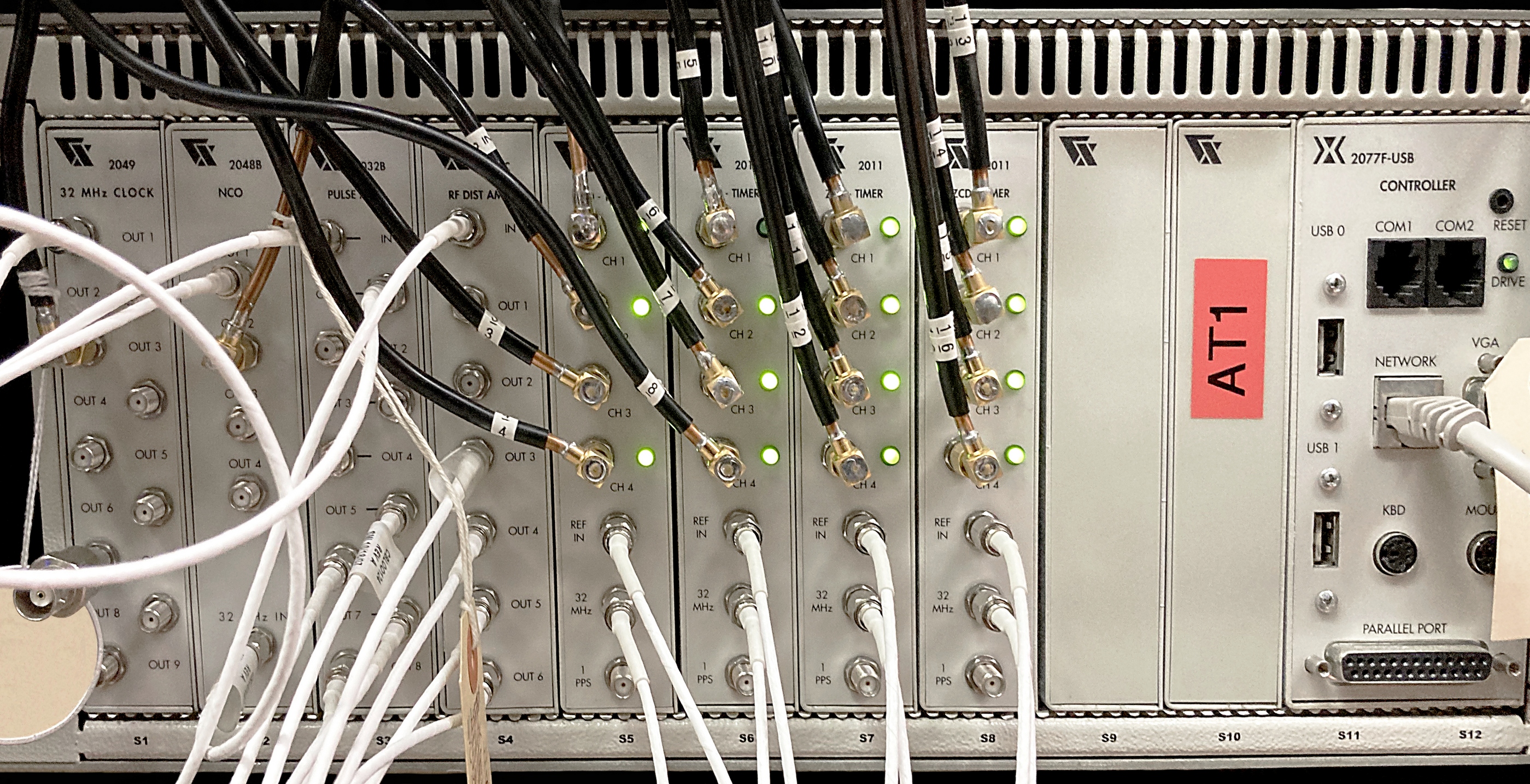
The Measurement Systems – To determine the phase differences and stability of each clock in the ensemble, one clock in the ensemble is arbitrarily chosen as a “pivot” clock, and each of the other clocks are continuously compared to the pivot clock every 12 minutes. These comparisons are made with a commercial multi-channel measurement system (MCMS). The signals from each atomic clock are routed to at least two MCMS units, with one designated as the primary system, and one or more alternate systems providing redundancy, as shown in Figure 4. Each MCMS unit can measure as many as 16 clocks via the dual-mixer time-difference (DMTD) measurement method. A photograph of an MCMS chassis is shown in Figure 5.
The measurement systems must be able to quickly detect very small frequency changes, and by use of the DMTD method, the MCMS can measure frequency stability to within < 1 × 10-12 at \( \tau=1\ s \). This is a much lower noise floor than other measurement devices such as time interval or frequency counters that are sometimes used in time scales. However, NIST is currently testing systems based on software-defined radio (SDR) techniques as an alternative to the MCMS. These systems potentially provide even lower noise floors, < 1 × 10-13 at \( \tau=1\ s \), and also offer the advantage of frequency agility. Diverse clock frequencies (for example not just 5 MHz but, in principle, any clock frequency) can be measured using the SDR technique, which will provide a significant advantage when optical atomic clocks are eventually integrated into the UTC(NIST) time scale.
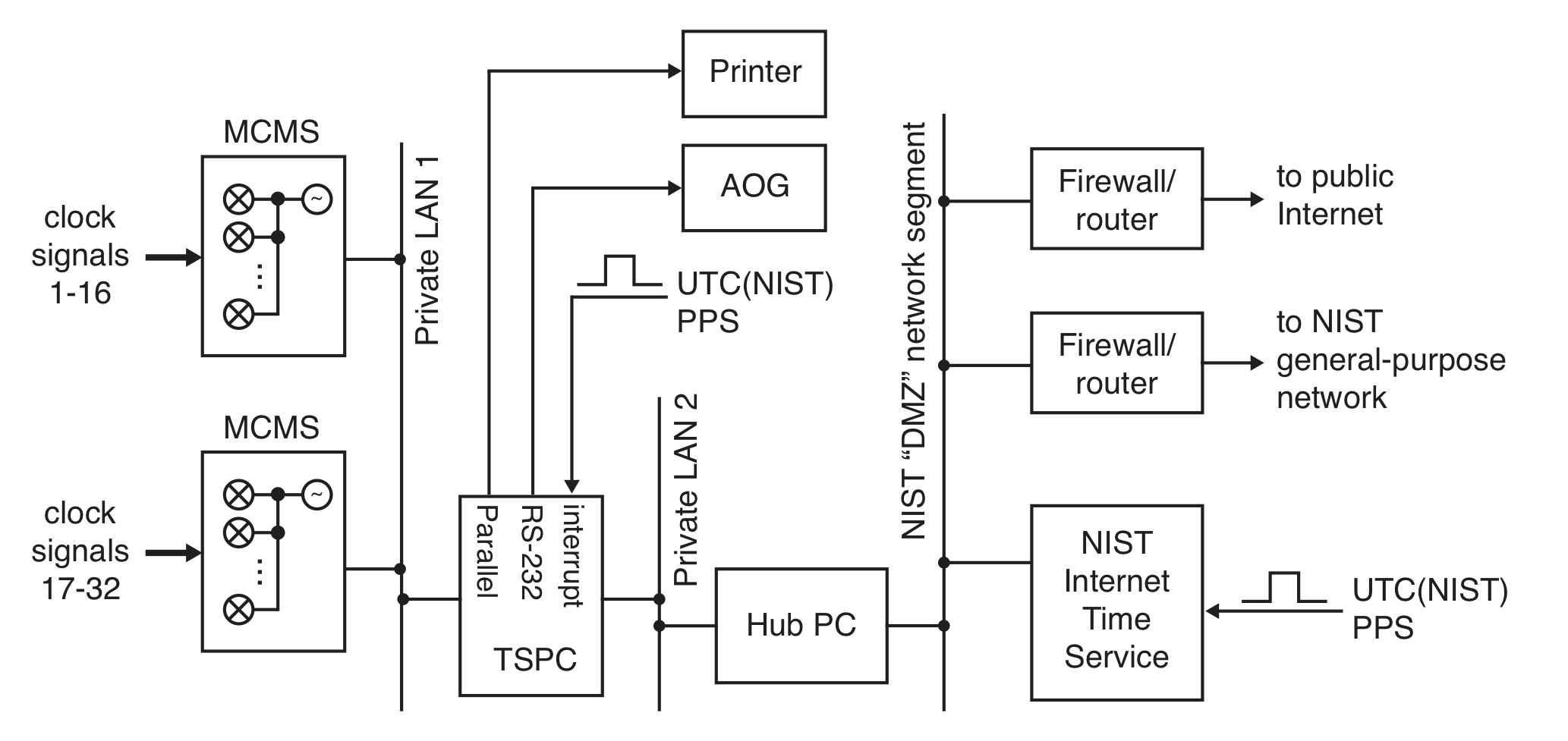
A dedicated time scale personal-computer (TSPC) continuously collects the clock data obtained from the MCMS units, as shown in Figure 6. As discussed in the following sections, the TSPC inputs the collected clock data into a time scale algorithm called AT1, and sends steering adjustments to an auxiliary output generator (AOG) that produces the physical UTC(NIST) signals. The TSPC is also connected to a hub computer that further analyzes and backs up data, tests for alarm conditions, and provides time-of-day information via connection to the NIST Internet Time Service (ITS).
The AT1 Algorithm and TA(NIST) - The free-running ensemble time scale TA(NIST) is controlled and adjusted by an algorithm called AT1, that attempts to make the TA(NIST) frequency as stable, predictable, and reliable as possible. Ideally, TA(NIST) performs better than its best clocks and is not made worse by including contributions from its worst clocks. Like many ensemble time scale approaches, AT1 uses signal averaging and the high frequency stability of atomic clocks to its advantage, even when the clocks lack absolute frequency accuracy.
The AT1 algorithm is complex, but essentially it works by averaging clock measurements to model the performance of each clock, and then using these models to predict each clock’s future behavior. For example, AT1 computes a moving average of each clock’s frequency offset. The averaging interval is made large enough (about 30 hours for hydrogen masers and about five months for cesium beam clocks) to reduce the effects of Gaussian noise, but not so large that other non-stationary noise processes become significant. In addition, AT1 determines the time difference and the linear drift rate of each clock. The clock time differences are measured every 720 seconds by the MCMS, with respect to a pivot clock as described earlier. A long moving-average (typically 7 to 15 days of averaging for masers and 31 days of averaging for cesium beam clocks) forms a model of expected time prediction error for each clock.
AT1 rewards the most stable clocks with the most weight when computing TA(NIST). Each clock’s stability is determined by repeatedly measuring its time difference with respect to the pivot clock. Then, weights are assigned to each clock in the ensemble based on their stability, with the total weights equaling 100%. To prevent a single clock from dominating the time scale, no clock can receive a weight of more than 30%. After the clock weights are determined, the time difference of the pivot clock with respect to the ensemble is computed as a weighted average. The weighting scheme makes sense, because the clocks with the best stability also have the smallest prediction errors, and thus contribute more to the determination of TA(NIST). If a clock’s time prediction error becomes larger than expected, its weight is decreased, and a clock whose weight has been decreased to 0 is removed from the time scale until its performance improves. A minimum of four clocks with a non-zero weight are required to keep TA(NIST) operational.
TA(NIST) is a virtual time scale that is defined in terms of its time difference with respect to each of the clocks in the NIST ensemble. It could be, but is not, realized as a physical signal. Instead, its output is combined with additional frequency and phase offset information to realize UTC(NIST), as described in the next section.
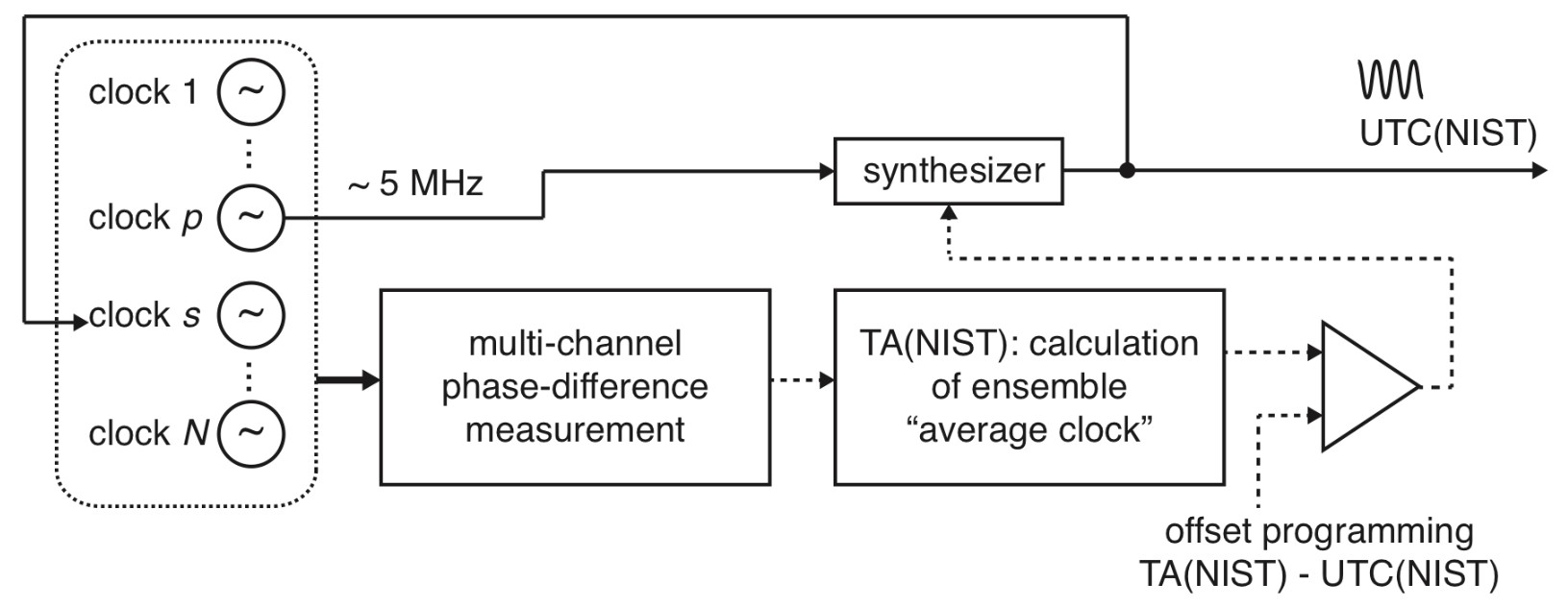
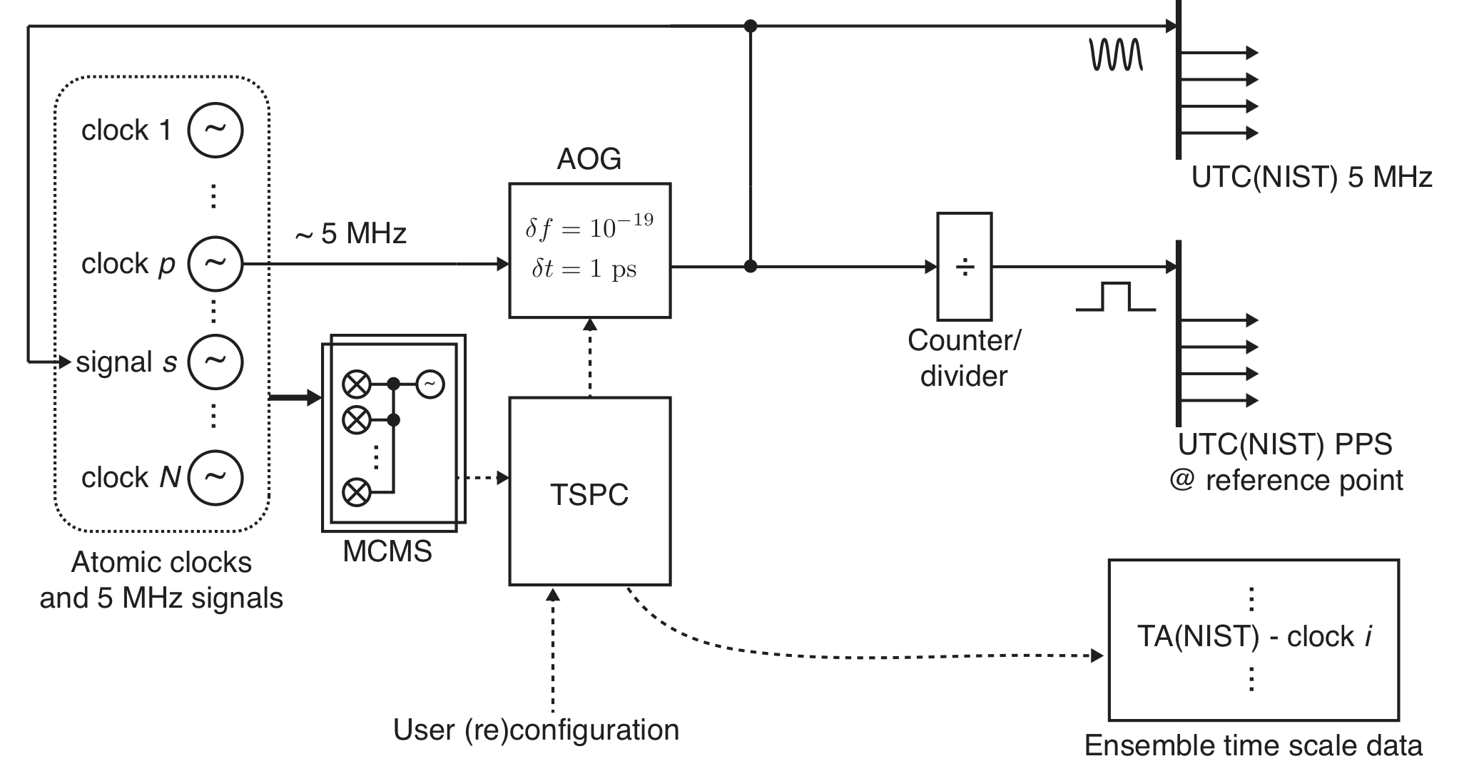
Realization and Generation of UTC(NIST) as a Physical Signal - UTC(NIST) realizes and generates physical signals through the use of a programmable, external synthesizer that is connected to the output of a free-running atomic clock, which is normally the pivot clock, clock p, that was discussed earlier. The synthesizer is then adjusted with corrections obtained from TA(NIST), as shown in Figure 7.
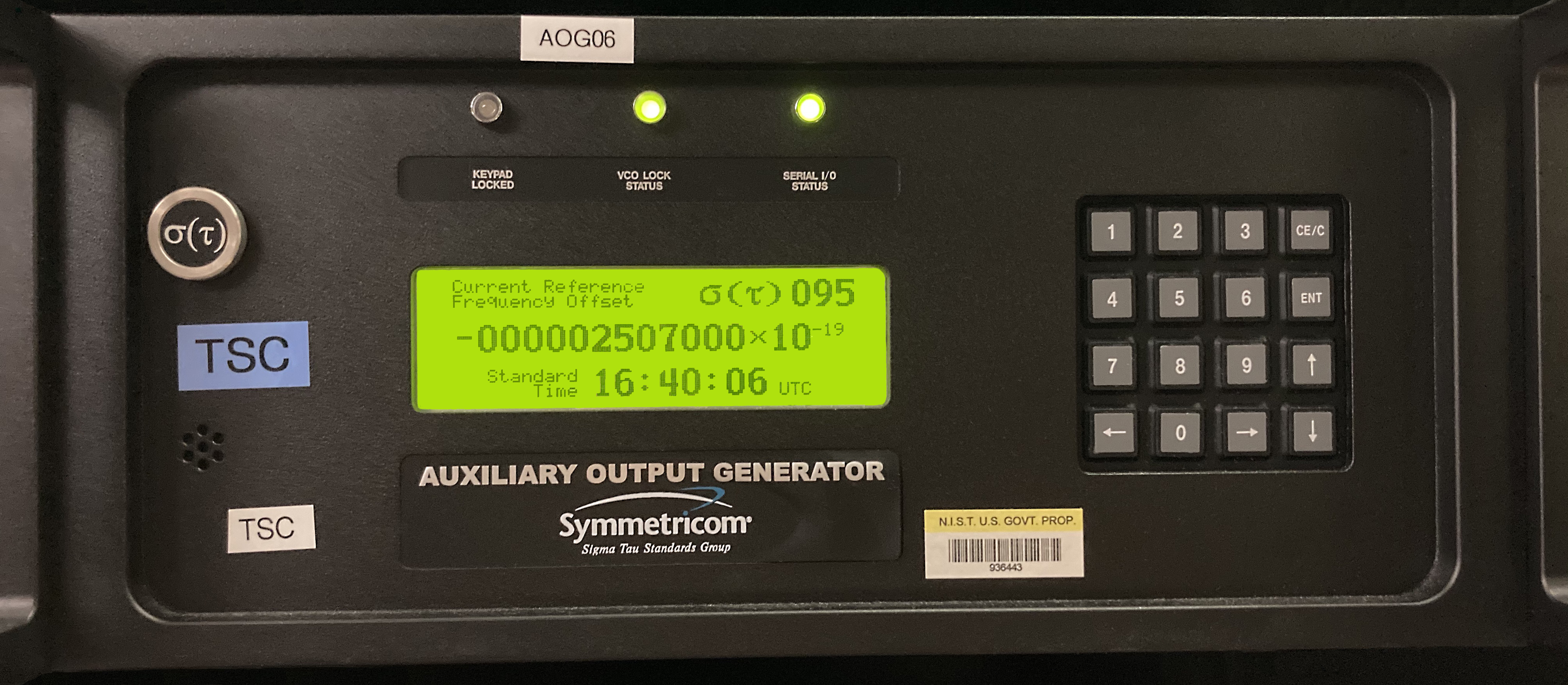
The external synthesizer approach has at least two major advantages. First, the BIPM only allows free running atomic clocks to contribute to UTC. By adjusting only an external synthesizer and allowing all of its clocks to free run, NIST keeps all of its atomic clock eligible for UTC contributions. The second advantage is that external synthesizers allow higher resolution frequency adjustments than the internal synthesizers found in individual atomic clocks. This allows the time scale output to be smoothly managed and controlled. For example, the output of the time scale can be smoothly adjusted by temporarily increasing or decreasing the programmed frequency offset for a fixed time interval, rather than by introducing a phase or time step. Figure 8 shows one external synthesizer utilized by NIST, known as an auxiliary offset generator (AOG). This device has a frequency resolution of 1 × 10-19 and a phase offset resolution of 1 picosecond.
The external synthesizer outputs a 5 MHz sine wave which is a physical expression of the frequency of UTC(NIST); a count of five million cycle of this frequency denotes a UTC(NIST time interval of 1 second. However, by convention, the absolute phase of this 5 MHz signal does not define UTC(NIST). Instead, the signal is routed to a counter/divider device also known as a pulse per second, or PPS generator (Figure 9).
The PPS generator works by employing a zero-crossing detector/amplifier and digital circuit to count 5,000,000 input cycles before triggering an output pulse and then resetting the counter. If the output pulse needs to be synchronized, for example if the time scale were to be restarted, internal procedures at NIST would bring the output pulse to within ±100 ns of UTC (half the period of 5 MHz); and closer synchronization would be accomplished by phase steering of the 5 MHz AOG signal.
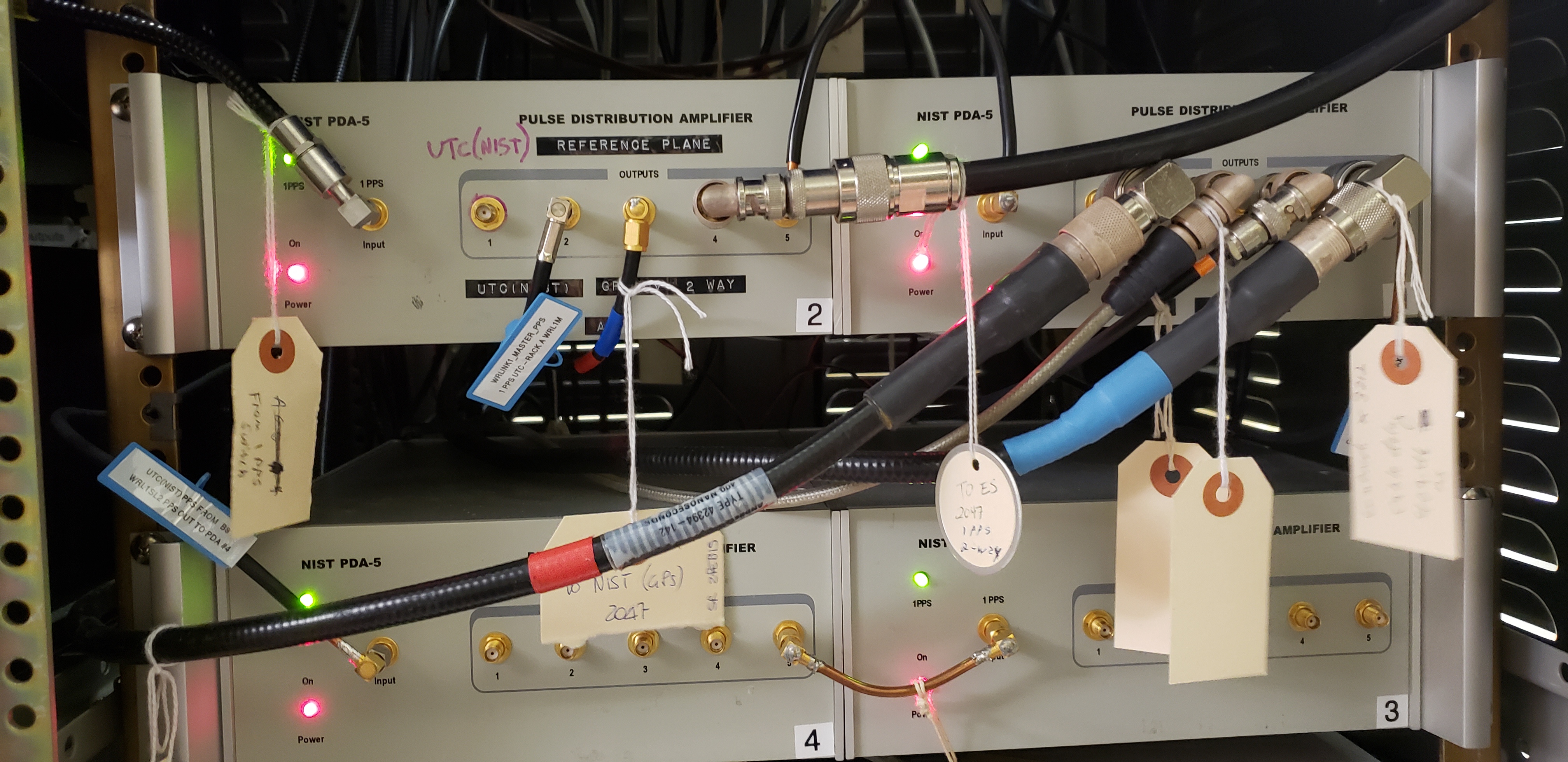
Following the counter/divider device, the generated PPS pulse is received at the input of a pulse distribution amplifier (PDA), as shown in Figure 10. By convention, a particular output connector of this PDA is defined as the UTC(NIST) reference plane. The pulses output at this connector represent the beginning of each SI second, and by counting these pulses NIST can indefinitely keep time.