
Official websites use .gov
A .gov website belongs to an official government organization in the United States.
Secure .gov websites use HTTPS
A lock (
) or https:// means you’ve safely connected to the .gov website. Share sensitive information only on official, secure websites.
SPC/E Water Reference Calculations - Non-cuboid Cell - 10Å cutoff
In this section, we provide sample configurations of SPC/E Water molecules [1] and report the various energy and force calculations for those configurations, where the coulombic contributions are computed using the traditional Ewald Summation Method [2]. These sample configurations and reference calculations can be used to validate the energy and force routines for an existing or new molecular simulation code. The discussion that follows places particular emphasis on the Ewald sum method for computing the Coulomb potential. The cutoff radius for real-space terms in this data set is 10Å.
All configurations described on this page are non-cuboid. Two of the configurations are triclinic, i.e. none of the lattice angles α,β,γ are 90°, and two configurations are monoclinic, i.e., α=γ=90° and β \= 90°. The lattice angles are given in the header of each sample configuration as described in the metadata file; the user can use the cell side lengths and lattice angles to generate either a lattice matrix or the "tilt" factors often used molecular simulation.
1. Periodic Boundary Conditions in Non-cuboid Cells
Application of periodic boundary conditions (minimum image convention) for non-cuboid simulation cells differs from that used for cuboid simulation cells. For description of the technique, consult the classic tutorial by W.R. Smith [3] or documentation of the LAMMPS molecular dynamics software [4].
2. SPC/E Model
The SPC/E Model represents water as a triatomic molecule with rigid bonds, i.e., both the length of the oxygen-hydrogen bonds and the angle between those bonds are fixed. The triatomic molecule has a single Lennard-Jones site centered on the oxygen atom and point charges centered on each atom:
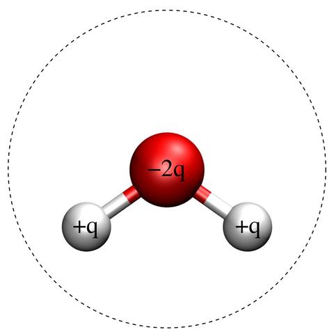
Fig. 1: Schematic of the SPC/E Molecule.
Red and white balls indicate oxygen and hydrogen atoms, respectively. The charges, indicated in the figure, are +q for both hydrogen atoms and -2q for the oxygen atom. The dashed line is a circle of diameter σ centered on the oxygen atom, signifying the effective size of the molecule. The hydrogen-oxygen bondlength is 1 Å and the hydrogen-oxygen-hydrogen bondangle is 109.47°. The remaining model parameters are [1]:
$$q = 0.42380~e $$
$$\sigma = 0.316555789~\textrm{nm}$$
$$\epsilon / k_B=78.19743111~K$$
3. SPC/E Potential Energy
The potential energy for the SPC/E model of water is:
$$ \Large E_{total}\left( \mathbf{r}^N \right) = E_{disp}\left( \mathbf{r}^N \right) + E_{LRC} + E_{coulomb}\left( \mathbf{r}^N \right) $$
The terms on the right hand side of the equality are the pair dispersion energy, the long-range correction to the pair dispersion energy, and the Coulombic potential energy, respectively. In the SPC/E Model, the pair dispersion energy is a Lennard-Jones intermolecular potential energy, which is discussed elsewhere in the NIST Standard Reference Simulation Website. The Coulombic energy is computed using the Ewald Summation Method, which is discussed below.
4. Ewald Summation Method
The Coulombic energy, and long-range energies, may be computed using the Ewald Summation Technique, which replaces the true Coulomb potential with the following [2,5]:
$$\Large \begin{eqnarray} E_{coulomb}\left(\mathbf{r}^N\right) & = & \dfrac{1}{2} {\sum\limits_{\mathbf{n}}}^{\dagger} \sum\limits_{j=1}^N \sum\limits_{l=1}^N
\dfrac{q_j q_l}{ 4 \pi \epsilon_0} \dfrac{\text{erfc}\left(\alpha \cdot \left| \mathbf{r}_{jl} + \mathbf{n}\right| \right)}{\left| \mathbf{r}_{jl} + \mathbf{n}\right|}\\
&& +\dfrac{1}{2 \pi V} \sum\limits_{\mathbf{k} \neq \mathbf{0}} \dfrac{1}{k^2} \exp \left[-\left( \dfrac{\pi k}{\alpha} \right)^2 \right] \dfrac{1}{4 \pi \epsilon_0} \cdot \left|\sum\limits_{j=1}^N q_j \exp \left(2\pi i \mathbf{k} \cdot \mathbf{r}_j \right) \right|^2 \\
&& - \dfrac{\alpha}{\sqrt{\pi}} \sum\limits_{j=1}^N \dfrac{q_j^2}{4 \pi \epsilon_0} \\
&& -\dfrac{1}{2} {\sum\limits_{j=1}^M}^{\dagger^{-1}} \sum\limits_{\kappa=1}^{N_j} \sum\limits_{\lambda=1}^{N_j} \dfrac{q_{j_\kappa} q_{j_\lambda}}{ 4 \pi \epsilon_0} \dfrac{\text{erf}\left(\alpha \cdot \left| \mathbf{r}_{j_\kappa j_\lambda} \right| \right)}{\left| \mathbf{r}_{j_\kappa j_\lambda} \right|}
\end{eqnarray}$$
The terms on the right hand side of the equality are 1) the real-space term Ereal, 2) the Fourier-space term, Efourier, 3) the self correction term Eself, and 4) the intramolecular term Eintra. We note that this form of the Ewald Summation 1) requires total charge neutrality for the configuration and 2) neglects the surface dipole term (equivalent to using the "tin-foil" or conducting surface boundary condition). The meaning of symbols in this equation are:
| n | Lattice vector of periodic cell images |
| k | Fourier-space vector of periodic cell images |
| k | modulus of k ; k2 = |k|2 |
| qj | Value of charge at site j |
| α | Ewald damping parameter |
| N | Total number of charged sites |
| M | Total number of molecules |
| Nj | Total number of charged sites in molecule j |
| κ, λ | Indices of sites in a single molecule |
| V | Volume of the simulation cell, LxLyLz |
| ε0 | Permittivity of vacuum (see below) |
| i | Imaginary unit, (-1)1/2 |
| rj | Cartesian vector coordinate of site j |
| rjl | rj -rl |
| erf(x) | Error Function computed for abscissa x |
| erfc(x) | Complimentary Error Function computed for abscissa x |
In this form, the superscript "†" (dagger) in Ereal indicates that the sum skips all pairs i=j inside the original simulation cell (n = 0). The superscript "†-1" in Eintra indicates that the sum is over site pairs within molecules in the original simulation cell. Additionally, the Fourier wave vectors (k) in this equation are composed of integer multiples of the basis vectors, e.g. k = 2u+v+4w where u, v, and w are the Ewald basis vectors [6]. The Fourier space term can alternatively be written using k vectors with elements proportional to 2π. In practice, the above equation is not how the Ewald Summation is actually implemented. Typically, one makes the following assumptions/reductions to simplify the summation:
- The real-space sum is done for the original simulation cell only, i.e. n=0.
- Site-site interactions in both Edisp and Ereal are truncated at a pre-defined cutoff rcut, where rcut ≤ min(Lx,Ly,Lz)/2. In practice, the damping parameter, α, is chosen so that contributions to the real-space term are negligible for rij > rcut.
- The Fourier space summation is truncated at a pre-defined maximum k or maximum value of k2.
Thus, the practical implementation of the Ewald Summation is [5]:
$$\Large \begin{eqnarray} E_{coulomb}\left(\mathbf{r}^N\right) & = &
\sum\limits_{j} \sum\limits_{l>j}
\dfrac{q_j q_l}{ 4 \pi \epsilon_0} \dfrac{\text{erfc}\left(\alpha \cdot \left| \mathbf{r}_{jl} \right| \right)}{\left| \mathbf{r}_{jl} \right|} \Theta\left( r_{cut} - \left|\mathbf{r}_{jl}\right| \right) \\
&& +\dfrac{1}{2 \pi V} \sum\limits_{\mathbf{k} \neq \mathbf{0}} \dfrac{1}{k^2} \exp \left[-\left( \dfrac{\pi k}{\alpha} \right)^2 \right] \dfrac{1}{4 \pi \epsilon_0} \cdot \left|\sum\limits_{j=1}^N q_j \exp \left(2\pi i \mathbf{k} \cdot \mathbf{r}_j \right) \right|^2 \\
&& - \dfrac{\alpha}{\sqrt{\pi}} \sum\limits_j \dfrac{q_j^2}{4 \pi \epsilon_0} \\
&& - \sum\limits_{j=1}^M \sum\limits_{\kappa} \sum\limits_{\lambda>\kappa} \dfrac{q_{j_\kappa} q_{j_\lambda}}{ 4 \pi \epsilon_0} \dfrac{\text{erf}\left(\alpha \cdot \left| \mathbf{r}_{j_\kappa j_\lambda} \right| \right)}{\left| \mathbf{r}_{j_\kappa j_\lambda} \right|}
\end{eqnarray}$$
We note that the real-space term now includes multiplication by the Heaviside Step Function, Θ(rcut - rij), which functionally truncates that term at rij = rcut.
The wave vectors in the Ewald sum are built from the Ewald basis vectors, which depend on the vectors that define the simulation cell. Calculation of the basis vectors and, ultimately, the wave vectors is described in the manual for DL_POLY Classic in section 2.4.5, "Ewald Sum." [6]
5. Parameters and Physical Constants for Reference Calculations herein
For the reference calculations given below, we use the following parameters and apply certain conditions to the calculation of both the dispersion interactions and the Ewald Summation:
| α | 0.2850/Å |
| kmax | 7 ; also only include k for which k2 < ksqmax. [See note below] |
| rcut | 10 Å |
| Truncation | |
| Dispersion | Truncate at rcut, apply analytic long-range corrections |
| Coulomb | Truncate real-space term at rcut |
| Boundary Conditions | Periodic and tin-foil (conducting) boundary conditions for all Cartesian Directions |
| erfc(x) | Implementation of Numerical Recipes ERFCC function; Ref. 7, page 164. |
The reference calculations given below were done using fundamental constants of physics and chemistry recommended by CODATA in 2018 [8,9]. We report these constants because the calculation of each contribution to the intermolecular energy will depend, ever so slightly, on the choice of fundamental physical constants and, in particular, the number of digits in those constants that are carried in the simulation. We use the full constants (untruncated) given in the CODATA 2018 recommendation:
| Name | Symbol | Value | Units |
| Boltzmann Constant | kB | 1.380649E-23 | J/K |
| Avogadro Constant | Na | 6.02214076E+23 | mol-1 |
| Planck constant | h | 6.62607015E-34 | J s |
| Elementary charge | e | 1.602176634E-19 | C |
| Permittivity of Vacuum | ε0 | 8.8541878128E-12 | C2/(J m) |
The Fourier-space term in the Ewald sum in sensitive to the number of wave vectors that are used. Most simulation packages reduce the number of wave vectors by discarding vectors whose square-length exceeds some pre-determined limit. For the calculations described in this page, the wave vectors included in the Ewald sum satisfy
$$k^2 < MAX\left[ \left( \dfrac{k_{x,max}}{lx} \right)^2, \left( \dfrac{k_{y,max}}{ly} \right)^2, \left( \dfrac{k_{z,max}}{lz} \right)^2 \right] $$
where lx, ly, and lz are the side lengths of the cell and kj,max is the maximum wave vector factor for the j direction. (In this example, kj,max = 7 for all Cartesian directions.) To aid reproducibility, the number of wave vectors used for each sample configuration is given in the table of Section 7.
6. Sample Configurations of SPC/E Water Molecules
Four sample configurations of SPC/E molecules are available for download as a gzipped tarball archive. This archive contains five files: the four sample configuration files and one metadata file that explains the format of the sample configurations. These configurations should be converted to the configuration file format native to a user's simulation software.
7. Reference Calculations of Intermolecular Energy for SPC/E
| Configuration -> | 1 | 2 | 3 | 4 |
| M (number of SPC/E molecules) | 400 | 300 | 200 | 100 |
| Cell Type | Triclinic | Monoclinic | Triclinic | Monoclinic |
| Cell Side Lengths [a, b, c] (Å) | [30 Å, 30 Å, 30 Å] | [27 Å, 30 Å, 36 Å] | [30 Å, 30 Å, 30 Å] | [36 Å, 36 Å, 36 Å] |
| Cell Angles [α, β, γ] (degrees) | [100°, 95°, 75°] | [90°, 75°, 90°] | [85°, 75°, 80°] | [90°, 60°, 90°] |
| Number of Wave Vectors | 831 | 1068 | 838 | 1028 |
| Edisp/kB (K) | 1.11992E+05 | 4.32860E+04 | 1.44033E+04 | 2.50251E+04 |
| ELRC/kB (K) | -4.10919E+03 | -2.10561E+03
| -1.02730E+03
| -1.63091E+02
|
| Ereal/kB (K) | -7.27219E+05 | -4.76902E+05 | -2.97129E+05 | -1.71462E+05 |
| Efourier/kB (K) | 4.46770E+04 | 4.44094E+04 | 2.88974E+04 | 2.23372E+04 |
| Eself/kB (K) | -1.15820E+07 | -8.68647E+06 | -5.79098E+06 | -2.89549E+06 |
| Eintra/kB (K) | 1.14354E+07 | 8.57652E+06 | 5.71768E+06 | 2.85884E+06 |
| Etotal/kB (K) | -7.21254E+05 | -5.01259E+05 | -3.28153E+05 | -1.60912E+05 |
Lastly, we note that we have reported six significant figures in each contribution to the intermolecular energy, while the software used for these calculations (a code written in FORTRAN) carried as many digits as possible within the specified machine precision. Thus, the reported Etotal may differ in the final digits from a user's calculation.
References
- H. J. C. Berendsen, J. R. Griger, and T. P. Straatsma, J. Phys. Chem., 91, 6269 (1987)
- P. Ewald, Ann. Phys., 369, 253 (1921)
- W. R. Smith, "The Minimum Image Convention in Non-Cubic MD Cells," (1989)
- LAMMPS Documentation, Section 8.2.2. "Triclinic (non-orthogonal) simulation boxes." Accessed October 29, 2021.
- M. P. Allen and D. J. Tildesley, Computer Simulation of Liquids (Oxford University Press, New York, 1989).
- W. Smith, T.R. Forester and I.T. Todorov, The DL POLY Classic User Manual (STFC Daresbury Laboratory, Cheshire, 2012). Accessed 3 November 2021.
- W. H. Press, et al., Numerical Recipes: The Art of Scientific Computing (Cambridge University Press, New York, 1986).
- E. Tiesinga, P. J. Mohr, D. B. Newell, and B. N. Taylor, Rev. Mod. Phys., 93, 025010 (2021)
- E. Tiesinga, P. J. Mohr, D. B. Newell, and B. N. Taylor, J. Phys. Chem. Ref. Data, 50, 033105 (2021)