e. Output

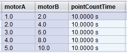
You can preview how the trajectory will run by hitting the Dryrun usa-button at the bottom of the panel. This will open a new window with the expected results.

The dryrun output matches the range and expression we created for motorA and motorB, respectively.

The positions for motorA correspond to the list we get from the range in our loop. The positions for motorB correspond to the list we get from the expression in our loop. The 10.0 seconds spent counting at each measurement state corresponds to the time preset we gave our counter in the Init section.

The above is an example of a point. Its measurement state is having motorA at position 1.0 and motorB at position 2.0 – and it counts at this measurement state for a duration of 10.0 seconds. However, because this is just a “mock” run, no data is written to disc or broadcast to listeners.

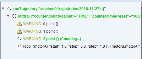
Once you’re ready to run a trajectory, hit the Run usa-button at the bottom of the panel.

You can see the trajectory running in the console queue – in the above example, the trajectory is at its third point, counting for the measurement state of motorA at position 3.0 and of motorB at position 6.0.

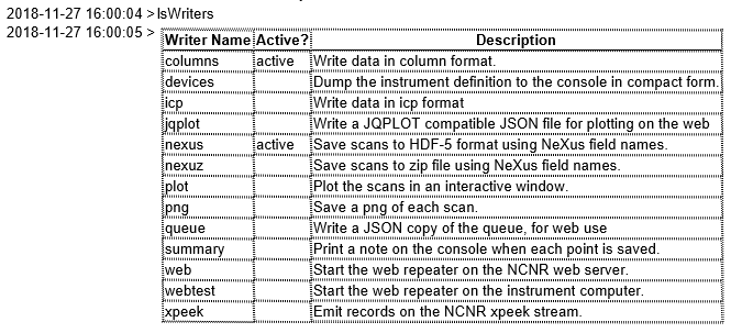
The console will print the estimated trajectory time and the location/name of the file(s) that was/were written. Multiple writers can be used to write multiple files in different formats. The lsWriters command displays a table of the available and active writers on the system. The table also contains short descriptions of each writer’s function, the data formats it uses, if/where data may be displayed, etc. The writer command starts and stops writers.

Note:    Files are written to /usr/local/nice/server_data/experiments/nonims()/data by default.