Official websites use .gov
A .gov website belongs to an official government organization in the United States.

Secure .gov websites use HTTPS
A lock ( ) or https:// means you’ve safely connected to the .gov website. Share sensitive information only on official, secure websites.

LAMMPS MD: Equation of State (pressure vs. density) - SPC/E Water

The main purpose of the following data set is to present equation of state (density-pressure-temperature) data for a version of the SPC/E Water fluid that was obtained using the LAMMPS Molecular Dynamics (MD) simulation suite. The secondary purpose of this data set is to provide sample LAMMPS input and initial configuration files that an end user may use in LAMMPS to obtain the same equation of state data, to either verify output from an installation of LAMMPS or educate the user about the basic features of LAMMPS. We first present output from LAMMPS, and compare it to Monte-Carlo derived results, and then provide a tutorial on how to reproduce that same data using LAMMPS.

Simulation details

Simulation Package	LAMMPS - see installation tutorial
Method	Canonical Ensemble (fixed N, V, T) Molecular Dynamics using the LAMMPS "nvt" ensemble option, with SHAKE constraints to preserve bond lengths and angles
Number of SPC/E Molecules	1500
Simulation Cell	Cubic cell, volume set with constant N=1500 to achieve desired reduced density
Truncation	Lennard-Jones Dispersion: 10 Å + analytic Long-range Corrections; Electrostatics: 10 Å + Long-range correction [either conventional Ewald or Particle-particle particle-Mesh (PPPM) Ewald]
Time Step	1.0 fs
Thermostat	Temperature imposed via Nosé-Hoover chained thermostats (three, LAMMPS default) with Tdamp=100 fs
Simulation length	1.1x10⁶ time steps (intended as 10⁵ equilibration steps followed by 10⁶ production steps)

Additional simulation details are in the sample input file, see below.

Results

1. Results for select temperatures (tabular)

The following table contains pressure and intermolecular potential energy per SPC/E molecule as a function of density for three temperatures, T=300, 400, and 500 K. The ensemble averages were calculated the LAMMPS runs described above and uncertainty, stated by the standard error, were estimated using block analysis (see below). For all three temperatures, phase stability is noted if applicable.

T = 300 K

T = 400 K

T = 500 K

ρ (kg/m³)

p (atm)

+/-

U/N (kcal/mol)

+/-

p (atm)

+/-

U/N (kcal/mol)

+/-

p (atm)

+/-

U/N (kcal/mol)

+/-

800

unstable

5.790E+01

2.938E+00

-8.362E+00

6.822E-04

850

unstable

5.521E+02

2.535E+00

-8.565E+00

8.531E-04

900

unstable

1.277E+03

2.659E+00

-8.758E+00

9.485E-04

950

unstable

5.109E+02

2.341E+00

-9.847E+00

3.753E-04

2.270E+03

2.550E+00

-8.934E+00

4.796E-04

990

unstable

1.358E+03

4.215E+00

-9.957E+00

8.887E-04

3.290E+03

2.992E+00

-9.064E+00

4.597E-04

995

unstable

1.479E+03

2.378E+00

-9.969E+00

7.589E-04

3.432E+03

3.951E+00

-9.078E+00

1.039E-03

1000

4.321E+01

5.118E+00

-1.674E+01

1.770E-03

1.599E+03

2.865E+00

-9.984E+00

1.050E-03

3.586E+03

2.888E+00

-9.095E+00

7.933E-04

1005

1.519E+02

5.504E+00

-1.117E+01

1.738E-03

1.732E+03

3.865E+00

-9.994E+00

7.756E-04

3.728E+03

2.868E+00

-9.108E+00

7.514E-04

2. Pressure-density-energy equation of state

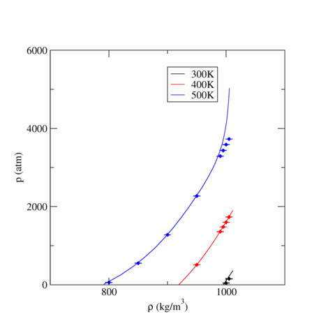
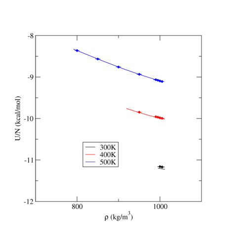
The following graphics show the pressure-density equations of state and the internal energy per molecule versus density in the form of a phase diagram for select temperatures (300, 400, and 500 K). In both graphics, the solid lines are the corresponding equation of state and energy as calculated from Grand Canonical-Transition Matrix Monte Carlo Simulations (GC-TMMC, see results elsewhere in the NIST SRSW). Solid symbols indicate the results from LAMMPS simulations, with the standard error shown by error bars. There is relatively good agreement between the two sets of results, except for the isotherm at 500K, which is approaching the critical temperature, where system-size effects are expected to lead to disagreement between different techniques.

Reproducing output

The LAMMPS MD results in the preceding table and graphics may be reproduced using example LAMMPS runs described as follows.

1. LAMMPS Installation

The data shown above were generated using a generic installation of LAMMPS, the executables of which may be reproduced as described here. This tutorial assumes some level of familiarity with POSIX-compliant operating systems (e.g., Unix, Linux, or Mac OSX) at the command-prompt level and access to a system with the GCC compiler, OpenMPI parallelization suite, Python, and the git version control system. This tutorial uses ">" to indicate the shell command prompt and $LAMMPS_DIR to identify the directory where LAMMPS is downloaded and later compiled. First, LAMMPS can be obtained using the instructions at http://lammps.sandia.gov/download.html#git via:

>git clone https://github.com/lammps/lammps.git

Second, LAMMPS executables may be compiled via:

   >cd $LAMMPS_DIR
   >git checkout stable_31Mar2017
>cd src
   >make purge
   >make package-update
>make yes-user-misc yes-molecule yes-rigid yes-kspace
   >make -j8 mpi

The installation sequence 1) switches to the "stable_31Mar2017" commit of LAMMPS (to ensure that a user is using the same code used to generate the data shown above), 2) removes any existing installation of LAMMPS, 3) updates any out of date packages, 4) installs the "USER-MISC", "MOLECULE", "RIGID", and "KSPACE" packages to enable the simulation of a rigid molecule using Ewald-type long-range electrostatics, and 5) builds an MPI-enabled executable using eight processor cores for parallel compilation. The end result is an executable named "lmp_mpi" located in the $LAMMPS_DIR/src directory.

Finally, we used the following operating system, compiler, and MPI libraries to build the LAMMPS executable:
Linux OS: CentOS 7; 3.10.0-514.21.1.el7.x86_64 kernel
   GCC: v4.8.5 (2015-06-23, listed as Red Hat 4.8.5-11)
   OpenMPI: v1.10.3 (2016-06-14)
   LAMMPS: Git Checkout Tag stable_31Mar2017 (2017-03-31)

2. Example LAMMPS Scripts

Example LAMMPS scripts and initial configurations that will yield the data shown above may be obtained from a git repository at: https://github.com/dwsideriusNIST/LAMMPS_Examples, e.g. via:

>git clone git [at] github.com:dwsideriusNIST/LAMMPS_Examples.git

This tutorial assumes that the git repository resides in $EXAMPLES_DIR. The relevant inner directories are:

SPCE_initial_cfgs	Initial configurations of N=1500 SPC/E molecules at the specified density i.e., spce_N1500_config.dens_800kgm3.lammps is an initial configuration at density ρ=800 kg/m³.
SPCE_reference_cfgs	Configurations of SPC/E molecules used for reference energy calculations. These configurations are identical to those used for Ewald summation reference calculations here and here.
run_scripts	Relevant LAMMPS Scripts
analysis	Python scripts to post-process LAMMPS output
SPCE_example	Example shell script that will run a LAMMPS simulation at ρ=1000 kg/m³

3. Example LAMMPS Run

A short example LAMMPS run is available in $EXAMPLES_DIR/SPCE_example, which may be run to confirm that LAMMPS is operating properly. This simulation is executed via:

>cd $EXAMPLES_DIR/SPCE_example
>sh example.sh

In the "example.sh" script, one can see that this script runs an SPC/E simulation at ρ=1000 kg/m³ and T=300 K for 60000 time steps (all LAMMPS settings are as shown previously, using the Particle-particle Particle-mesh k-space option) then analyzes the MD trajectory to report the average temperature, pressure, and potential energy. The final output, from the block analysis script, will report the following ensemble averages and uncertainty:

Thermodynamic Ensemble Averages from: ave.dens_1000kgm3.out
Discarded Timesteps: 10000
Number of Blocks: 5
Block size (timesteps): 10000
Stated uncertainty is the standard error of the thermodynamic property

Temperature +3.0011E+02 +/- +1.5853E-01
PotentialEnergy -1.6730E+04 +/- +8.4612E+00
Pressure +3.6834E+01 +/- +2.9068E+01

4. SPC/E Reference Energy Calculations using LAMMPS

NIST provides reference energy calculations for SPC/E configuration elsewhere in the Standard Reference Simulation Website (9 Å cutoff and 10 Å cutoff); those calculations were made using a custom implementation of the Ewald summation. Here we provide a script that can recreate those reference calculations using LAMMPS, with some modifications. The git repository referenced earlier contains the four SPC/E configurations from the SPC/E reference calculations in LAMMPS format, as files spce_sample_config_periodic_cubicN.LAMMPS, with "N" replaced with 1, 2, 3, or 4. The energy of one of these configurations, using the 9 Å cutoff, may be computed via:

>cd $EXAMPLES_DIR

>mkdir ref_energy ; cd ref_energy

>cp ../run_scripts/SPCE.initial_energy ./ ; cp ../SPCE_reference_cfgs/spce_sample_config_periodic_cubic1.LAMMPS ./

>mpirun -np 12 lmp_mpi -in SPCE.initial_energy -var infile spce_sample_config_periodic_cubic1.LAMMPS

The reference energies, separated into the pair dispersion, dispersion long-range correction, real-space coulombic, and Fourier-space coulombic terms are given in Table 1.

Table 1: SPC/E Reference energy, by term, calculated using LAMMPS

Configuration ->	1	2	3	4
Number of SPC/E Molecules	100	200	300	750
Pair Dispersion (kcal/mol)	1.984342E+02	3.873873E+02	7.096428E+02	9.012683E+02
Dispersion Long-range Correction (kcal/mol)	-2.244726E+00	-8.978904E+00	-2.020253E+01	-3.741210E+01
Real-space Coulombic (kcal/mol)	4.473370E+03	8.797163E+03	1.285080E+04	2.126526E+04
Fourier-space Coulombic (kcal/mol)	-5.640534E+03	-1.129400E+04	-1.694854E+04	-2.824985E+04
Total Energy (kcal/mol)	-9.709749E+02	-2.118424E+03	-3.408305E+03	-6.120733E+03

The reference calculations here are presented with more granularity (separation of the real-space and Fourier-space terms) and must be modified slightly for comparison with LAMMPS. Specifically, the LAMMPS Real-space Coulombic term is equal to E_real + E_intra and the LAMMPS Fourier-space Coulombic term is equal to E_fourier + E_self. Also, the units must be converted from Kelvin units to kcal/mol, which was done using the CODATA 2010 set of physical properties. The results are shown in Table 2.

Table 2: SPC/E reference energies from "SPC/E Water Reference Calculations - 9Å cutoff", converted to LAMMPS-equivalent terms and units.

Configuration ->	1	2	3	4
Number of SPC/E Molecules	100	200	300	750
Pair Dispersion (kcal/mol)	1.984342E+02	3.873874E+02	7.096430E+02	9.012686E+02
Dispersion Long-range Correction (kcal/mol)	-2.244727E+00	-8.978906E+00	-2.020254E+01	-3.741211E+01
Real-space Coulombic (kcal/mol)	4.473373E+03	8.797168E+03	1.285080E+04	2.126529E+04
Fourier-space Coulombic (kcal/mol)	-5.640523E+03	-1.129397E+04	-1.694853E+04	-2.824984E+04
Total Energy (kcal/mol)	-9.709607E+02	-2.118396E+03	-3.408283E+03	-6.120694E+03

There are minor differences between the two sets of calculations, which follow from 1) different truncation schemes for physical parameters, 2) different implementations of the complementary error function, 3) different strategies for selecting the number of k-vectors, and 4) floating-point precision.

5. Production LAMMPS Runs

Production LAMMPS runs to generate SPC/E equation of state data may be run using the scripts provided in $EXAMPLES_DIR/run_scripts and the initial configurations in $EXAMPLES_DIR/SPCE_initial_cfgs. Syntax for execution of a run is:

>mpirun -np $NP lmp_mpi -in SPCE.NVT -var infile $FOO -var temp $BAR

where $NP is the number of processors to utilize, $FOO is the specified initial configuration, and $BAR is the absolute temperature (in K units). We note that the initial configuration file (e.g., spce_N1500_config.dens_1000kgm3.lammps) must be in the run directory. Block Analysis of the results may be done via the script provided in $EXAMPLES_DIR/analysis:

>$EXAMPLES_DIR/analysis/block_analysis.py -f $FILENAME -b $BLOCKS -m $STEPS_SKIP

where $FILENAME is the LAMMPS output file containing MD trajectory data, $BLOCKS is the number of blocks to use for uncertainty analysis, and $STEPS_SKIP is the number of timesteps from the start of the simulation to discard (i.e., "equilibration" timesteps).

Lastly, an example production run at T=300 K, ρ=1000kg/m³, using 12 processors may done via:

>cd $EXAMPLES_DIR

>mkdir test ; cd test

>cp ../run_scripts/SPCE.NVT ./ ; cp ../SPCE_initial_cfgs/spce_N1500_config.dens_1000kgm3.lammps ./

>mpirun -np 12 lmp_mpi -in SPCE.NVT -var infile spce_N1500_config.dens_900kgm3.lammps -var temp 300.0

Based on the input file, this simulation will run for 1.1x10⁶ time steps, and produce a MD trajectory file named ave.out. The trajectory may be analyzed (discarding the first 100000 timesteps and using 10 blocks to estimate the uncertainty in the remaining 1000000 timesteps) via:

>../analysis/block_analysis.py -f ave.out -b 10 -m 100000

The final output is:

Thermodynamic Ensemble Averages from: ave.out
Discarded Timesteps: 100000
Number of Blocks: 10
Block size (timesteps): 100000
Stated uncertainty is the standard error of the thermodynamic property

Temperature +2.9998E+02 +/- +2.8905E-02
PotentialEnergy -1.6744E+04 +/- +1.7701E+00
Pressure +4.3206E+01 +/- +5.1179E+00

The reported ensemble averages are the (kinetic) temperature in Kelvin, the internal energy in kcal/mol, and (virial) pressure in atmospheres. The results shown are identical to those for T=300 K and ρ=1000kg/m³ in the previous table. Finally, we note that these results will be generated exactly as shown provided that the number of parallel processors is set to 12. Choosing a different number of processors will affect the resultant ensemble average and uncertainty due to differences in the random number generator in LAMMPS as well as round-off truncations.

Chemical thermodynamics and chemical properties, Thermodynamics and Reference data

Contacts

Daniel W. Siderius

daniel.siderius@nist.gov

(301) 975-5968

Created July 6, 2017, Updated March 12, 2025