Research Updates – Gas Flow for Semiconductor Manufacturing

07 March, 2023

NIST’s Rate of Rise Flow Standard (RoRFS)

In our last post, we described the preliminary design of NIST's Rate of Rise Flow Standard (RoRFS) being developed to calibrate semiconductor meters for flows ranging from Q̇ = 0.01 sccm to 1000 sccm at a target expanded uncertainty of 0.1 % or less. This blog 1) provides additional details on the design, 2) illustrates how mass flow is determined, 3) introduces a physical model that characterizes the increase in gas temperature in the collection tank attributed to flow work, 4) compares the measured pressure spike used to determine the temperature with the spike predicted by the physical model, 5) updates the RoRFS collection tank design, and 6) shows tests of the repeatability/reproducibility of a scaled RoRFS using SF₆ and N₂ for flows at approximately 150 sccm.

Design Details

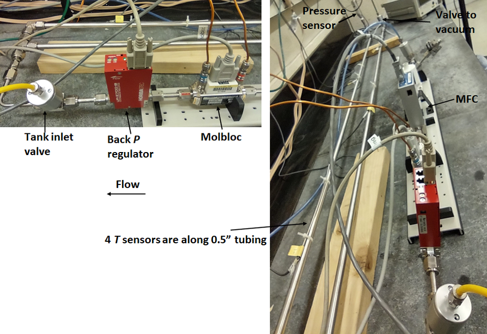
The primary components of the RoRFS are shown in Figure 1 and include 1) the gas source; 2) a mass flow controller (MFC) to establish a constant mass flow; 3) the meter under test (MUT) being calibrated; 4) pressure regulators; 5) a long, slender collection tank of known volume (V_tank); 6) a vacuum pump downstream of the collection tank; 7) pressure and temperature sensors; and 8) valves to start/stop flow and partition the collection tank or other parts of the standard; 9) a thermostatted enclosure (not shown in the figure) that recirculates air at constant temperature T_∞ over the MUT piping and the collection tank.

The design of the collection tank depicted in Fig. 1 illustrates our strategy for limiting flow work related heat transfer effects. Our temperature model discussed later in the blog shows that the long tubing promotes heat transfer, facilitating fast thermal equilibrium of the gas in the tank both during the filling process and after the tank inlet valve is closed and flow stops. Although the schematic in Fig. 1 shows a specific design consisting of N_tubes = 6 finned tubes connected in series, this is not the configuration we have decided to use in our first full size flow standard (we are not sure if it will be the final version at this time). The configuration and design consideration are discussed below in the section about updates to the RoRFS collection tank design. For clarity, experimental results specify these design parameters and provides the tube dimensions D_i and L_tube. The results presented for our bench top standard are with the tubes configured in parallel.

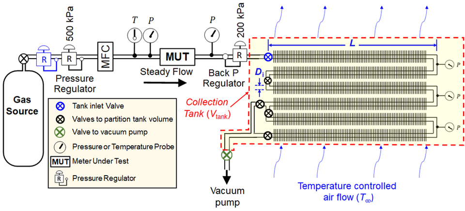
During calibration, the MUT measures the constant mass flow ṁ_MUT established by the MFC. The steady flow exiting the MUT accumulates in the collection tank. A regulator installed immediately downstream of the MUT isolates the MUT from the rising gas pressure in the tank. As the gas enters the collection tank it compresses the existing gas so that the temperature increases during the filling process (i.e., the flow work phenomenon). Accurately measuring this changing temperature with a probe is challenging due to the poor heat transfer between the probe and the nearly stagnant gas. As a result, the RoRFS does not use temperature probes inside in the collection tank. Instead, we measure the temperature T_∞ of thermostatted air outside of the collection vessel and determine the temperature increase ΔT of the gas inside the vessel caused by a balance of flow work and heat lost through the vessel wall to the environment. We determine ΔT by measuring the pressure spike that occurs immediately after the flow is stopped (see Fig. 4). After the flow is stopped, the mass and the average gas density in the collection tank remain constant. Accordingly, changes in pressure correlate with temperature as the temperature relaxes back to T_∞. We exploit this correlation to determine ΔT, and subsequently, the temperature in the collection tank during filling,

How Mass Flow is Determined

Conservation of mass stipulates that the rate of mass accumulation in the collection tank equals the mass flow,

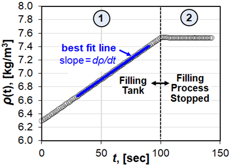
which is equal to the product of the collection tank volume (V_tank) and the rate of change of the density (dρ/dt). Figure 2 shows the increase in the density of SF₆ gas nominally flowing into the collection tank at Q̇ = 163.2 sccm. A NIST traceable equation of state for SF₆ calculates the density ρ = ρ(P, T) at each point (○) as a function of the measured pressure P and the steady state temperature T given in Eq. (1). The rate of change of the density is determined using the slope of the line (──) depicted in Figure 2. Since ρ is determined using the steady state temperature, the slope of the density must be calculated after temperature transients have dissipated when ρ varies linearly with time. We estimate the time required to reach steady state using our temperature model discussed in the next section. In addition, we check that the linear regression of the density versus time data yields an uncertainty of the slope that is no more than 0.01 % at the 95 % confidence level. If the selected data used to compute the slope does not satisfy this criterion, the tank is evacuated, and the filling process is repeated.

Temperature Model

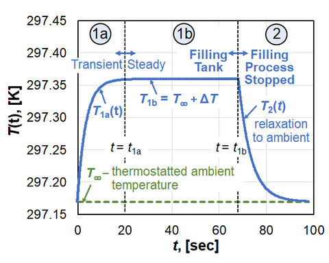
We developed a physical model based on mass and energy conservation to predict the gas temperature in the collection tank throughout the calibration process. This model is important because it tells us when the data is acceptable to calculate the slope of the mass vs. time, i.e., that the temperature has reached the steady state value during filling. The results of the model are illustrated by the two temperature traces shown in Fig. 3. The dashed line (----) shows the constant temperature T_∞ of the thermostatted air outside the collection tank while the solid line (──) shows the gas temperature T inside the tank. These temperature traces are depicted during two periods: 1) the period during flow when mass accumulates in the collection volume, and 2) the period after the flow stops and M_tank is constant. The dashed vertical line (----) at t = t_1a divides the filling period into 2 intervals. The interval t < t_1a shows the transient gas temperature T_1a that increases above T_∞ to the steady state temperature T_1b due to flow work. The slope of the density in Fig. 2 is calculated after the time t_1a predicted by the model. For the interval t ≥ t_1a the heat generated by flow work is balanced by heat loss through the collection tank walls so that T_1b = T_∞ + ΔT is nearly constant. The model predicts the temperature increase due to flow work is

where ṁ is the mass flow, the gas constant R_gas =R_univ/M is the ratio of the universal gas constant and the molar mass of the semiconductor gas; k is the gas thermal conductivity, L_tube is the length of the collection tank tube(s); and N_R is a virial correction parameter that is generally close to unity. Historically, the semiconductor industry expresses mass flow in volumetric units at standard, or reference conditions of P_REF = 101.325 kPa and T_REF = 273.15 K. To accommodate readers familiar with this notation, the mass flow in Eq. (3) is expressed as a standard volumetric flow, ṁ = ρ_REF Q̇. Here, ρ_REF = ρ(P_REF, T_REF) is the density of the gas evaluated at standard pressure and temperature using the REFPROP database.  

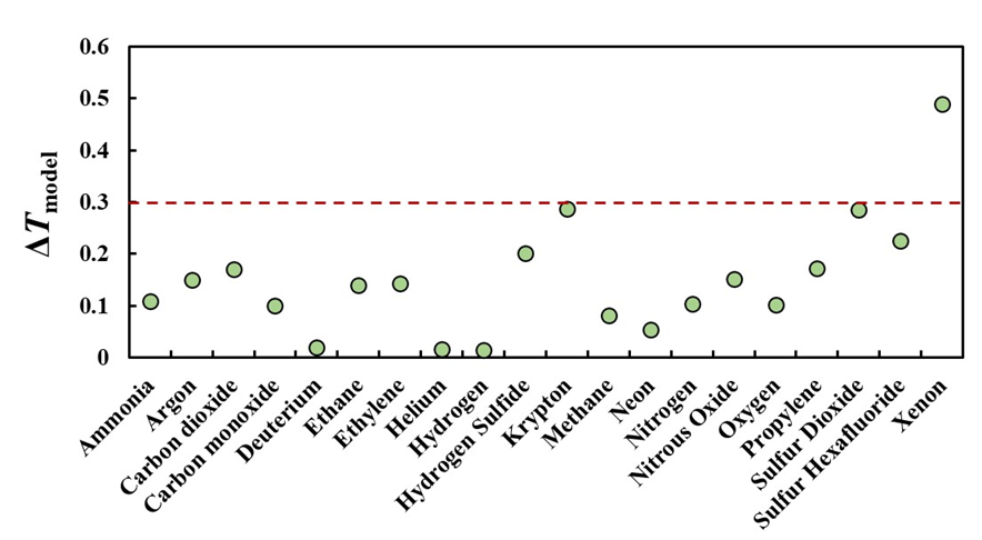
We use Eq. (3) to support the design of the collection tank. For example, the gas species dependence of ΔT depends solely on the thermodynamic and transport properties expressed by

$$\frac{N_{R}ρ_{REF}R_{univ}}{(Mk)}$$

in Eq. (3). For a specified flow Q̇ accumulating in the collection tank consisting of tubes of length L_tube with thermostatted air at T_∞, the temperature increase ΔT depends only on the gas properties of the semiconductor gas. For a given tank volume, one can decrease ΔT by increasing the length L_tube of the tubes comprising the collection tank. Using this strategy, we designed our collection tank so that the maximum temperature increase due to flow work is less than ΔT_max  ≤ 0.3 K for the majority of the gasses we plan to investigate. To realize the desired temperature criterion, we plan to design a collection tank with N_tubes = 16 each having D_i = 0.010 m and L_tube = 1.8 m for a total length of 29.28 m, and the maximum flow is Q̇ = 1000 sccm. Figure 4 shows ΔT for many semiconductor gases. We would need 26 tubes to achieve a 0.3 K change for xenon gas. This would lead to a significantly longer collection time for the other gases and is not seen as a necessity at this time. Note that the uncertainty in the temperature measurement will be much smaller than ΔT: we will measure the pressure spike and apply our physical model to correct for the flow work effects on the temperature measurement.

Comparison of the Model to Experiment

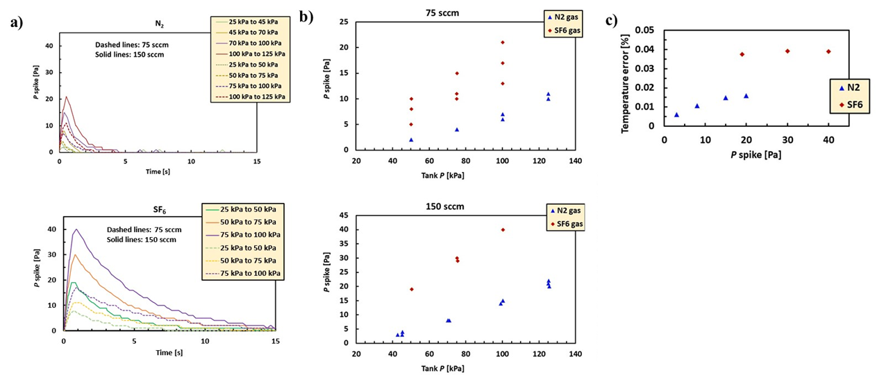
Figure 5 shows some example pressure spikes measured in our benchtop standard. These spikes indicate the measured room temperature is 0.04 % and 0.07 % different from the internal gas temperature during filling for N₂ and SF₆ gas, respectively. This is a correction we can easily make. We tested our model against experimental data for the original planned tube size for our collection volume (D_i = 0.021 m, or 0.825 in) and the revised tube size (D_i = 0.010 m, or 0.3925 in) since the last blog post. L_tube = 1.8 m and the tubes are configured in parallel. Figure 5 shows the results for a flow of ≈ 150 sccm of N₂ and SF₆ in both tube sizes. The model (──) predicts the measured pressure spike (○) within 15 % for our maximum flow of N₂ and SF₆. This corresponds to a maximum expanded uncertainty in the gas T of 0.015 %. The temperature uncertainty will be much lower for smaller flows where the flow work is minimal and ΔT < 0.3 K.

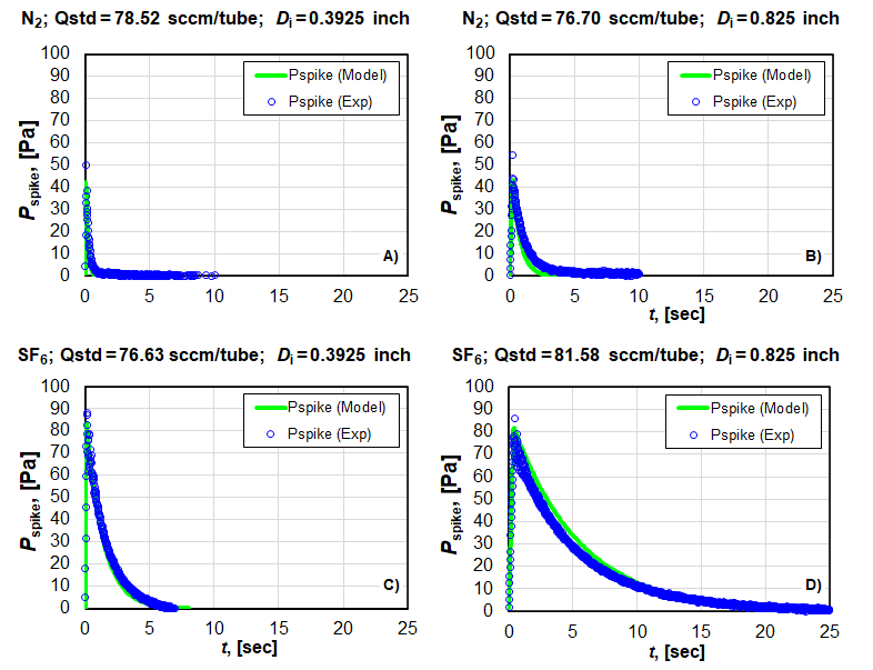
It is important to notice the time it takes to reach thermal equilibrium once the flow is stopped in Fig. 5 for the two different tube diameters. Because the volume of collected gas is less in a tube of the same length but smaller diameter, the time for it to reach equilibrium is less. This is also true with respect to the time it takes to equilibrate when filling begins as discussed above. It is desirable to have the gas reach equilibrium quicker when filling because that allows the collection of more data points to reduce the error in the slope calculation. However, it is also important that the pressure spike is well-resolved in order to make an accurate temperature correction: it may be hard to measure its true magnitude if the response time of the pressure sensor is too low. We have decided to use tubing with a nominal diameter of 1.27 cm (measured D_i = 0.010 m, or 0.3925 in). We believe this is the lower limit to obtain adequate resolution of the pressure spike.   

Updates to the RoRFS Design

Since our last post, the FMG has decided 1) to reduce the size of the collection volume, 2) eliminate the fins on the tubes, and 3) plumb the tubes in series. Modeling of flow work produced while filling the tubes and experimental results show that we do not need the large volume of 15 L originally planned; 2.4 L will provide sufficient filling time. Therefore, we will use tubing with D_i = 0.010 m. We will plumb 16 tubes, each with L_tube = 1.8 m in series to make the final volume of 2.4 L with L = 29.3 m. 

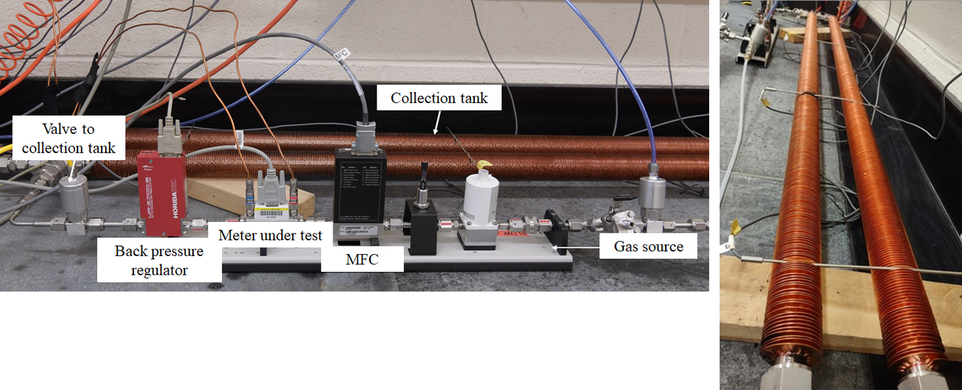
We plumbed two of the smaller diameter tubes together in parallel for a revised benchtop standard with V  ≈ 0.363 L  (Fig. 6) and the data presented below is from that arrangement. Our benchtop standard is a factor of 8 smaller than our planned volume and the maximum scaled flow is 150 sccm. (1000 sccm is our planned maximum flow in the final volume.) Prior testing showed that the fins are not necessary, and we decided to plumb the tubes in series because it is much easier than parallel.

In addition to reducing our collection tank volume, we replaced a pressure sensor that has a response time of ≈ 6.2 Hz with one with a response time of ≈ 52 Hz. This allowed us to better resolve the pressure spike and better determine ΔT, which allowed us to physically model the heat transfer in the tank as discussed above.

We verified our new volume will give us an acceptable amount of data points over the flow range of 1 sccm to 150 sccm. This is important for the fit to the calculated gas density vs. time to determine the gas flow. The pressure and temperature sensors have inherent noise. We need enough data that the fit of a straight line gives acceptable uncertainty. We can achieve 95 % uncertainty in the slope of this line within 0.01 %.

Repeatability/reproducibility of a scaled RoRFS

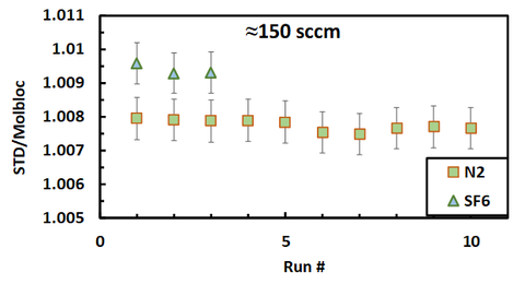
We have begun to validate our benchtop standard using a molbloc and N₂ and SF₆ gas. Figure 7 shows the meter factor, the ratio of the flow determined by the standard to that reported by the meter. We compared repeated rate-of-rise measurements and the molbloc at ≈ 150 sccm. No sensors were calibrated and hence this test only measures the repeatability of our standard. The meter factor, i.e., the flow according to the standard divided by the flow measured by the molbloc is plotted on the y-axis. For N₂, five measurements

were made sequentially. Then the flow was turned off, restarted, and five more measurements were collected, giving a total of ten total measurements. For SF₆, three measurements were made sequentially. The standard deviation of the 10 N₂ meter factor measurements is 0.02 %, which is the same for the 3 SF₆ meter factor measurements. This shows the benchtop RoRFS has repeatability that is more than adequate for our purposes. The error bars are 0.05 % of the meter factor, which is our target k = 2 uncertainty for inert gases with known properties. It should be noted the meter factor is different for the two gas species. This is the reason for undertaking for this work: to measure and model the gas property effects on the flow meters used in chip fabrication 

Our next step is to weld together 16 of the nominal 1.27 cm diameter tubes in series to achieve our final volume. We will then place this volume in a temperature-controlled enclosure. In a future blog we will described the RoRFS thermostated enclosure (still under construction) and describe its effectiveness maintaining constant surface temperature on the outer surface of the collection tank during the calibration process. While the thermal enclosure is being completed, we measure T_∞ by averaging readings from 4 thermistors spaced axially along the length of the collection tank tubing (Fig. 6). Each thermistor measures the air adjacent to the tube wall every 1.5 s throughout the calibration process.

---

08 December, 2022

The Fluid Metrology Group (FMG) has begun the design and construction of a semiconductor gas flow standard. It will use the rate of rise technique, in which the rate of change of gas density in a collection volume measured over time gives the mass flow. Figure 1 shows a prototype for the flow standard, which is approximately an order of magnitude smaller in volume than the target design. We call this our benchtop standard.

We have procured finned tubes as shown in Fig. 1 for a collection volume. The tubes are 1.85 m long and have an outer diameter of 0.0254 m. The original plan was to use 16 of them for a final volume of approximately 15 L. However, final tube size, shape, and number will be determined from our benchtop standard. Our maximum planned flow is 1000 sccm, which is equivalent to 150 sccm when scaled for our smaller benchtop standard. In addition to building a standard to measure semiconductor gas flow, we are working closely with NIST’s Thermophysical Properties of Fluids Group to determine gas properties for gases used in semiconductor manufacturing. The FMG has previously measured properties of some semiconductor gases, which can be found here.

To accurately measure the density as the collection tank is filling, we must be able to measure the incoming gas temperature and pressure with appropriate response time and resolution and have an equation of state to calculate the density from these inputs. Currently, the FMG has a rate of rise gas flow standard for inert gases with well-known equations of state. The collection volume is submerged in a well-stirred, temperature-controlled water bath whose temperature we measure. We do not measure the temperature of the gas in the volume directly. As the collection tank fills, heat generated in the gas by flow work will be balanced by the heat transfer to the water bath, i.e., the gas temperature will rise above that of the water temperature. For low flows, this gas temperature rise is negligible, but as the flow is increased, the gas temperature increase produces an error in the calculated density and must be corrected. This phenomenon produces a “pressure spike” when the flow is stopped as shown in Fig. 2. Because water is corrosive and a large water bath is difficult to maintain, we are testing whether a temperature-controlled air bath will work instead. With sufficient heat transfer, the difference between the temperature of the gas in our full collection volume and the air bath will be insignificant. Alternatively, if the temperature error is predictable, we can make the necessary correction.

We have measured the magnitude of the pressure spike (and hence the temperature error caused by flow work) in our benchtop standard using nitrogen and sulfur hexafluoride gases with and without air blowing across the finned tubes. We chose these two gases because they have very different heat capacities and thermal conductivities [C_p/C_v = 1.4 for N₂ and 1.1 for SF₆, thermal conductivity = 25.24 mW/(m-K) for N₂ and 12.38 mW/(m-K) for SF₆]. We see no effect on the magnitude of the pressure spike when a large fan is used to flow air across the tubes. This means our heat transfer is limited by the heat transfer inside the collection volume, so now we are investigating designs that improve the internal heat transfer. In a future update, we will discuss some theoretical models that describe the thermodynamics during the filling process that predict the temperature error to guide our design effort.