
Official websites use .gov
A .gov website belongs to an official government organization in the United States.
Secure .gov websites use HTTPS
A lock (
) or https:// means you’ve safely connected to the .gov website. Share sensitive information only on official, secure websites.
LFPF Software
The Logistic Function Profile Fitting program, LFPF, is based on a Fortran program written for DOS and originally issued under the name LOGIT. This program was successfully used to fit Auger sputter-depth-profile data [W. H. Kirchhoff, G. P. Chambers, and J. Fine, J. Vac. Sci. Tech. A 4, 1666 (1986)]. This approach and the associated software were applied in a number of laboratories, and formed the basis for ASTM standard E 1636-10: Standard Practice for Analytically Describing Sputter-Depth-Profile Data by an Extended Logistic Function. The logistic function (although not the specific LOGIT or LFPF software) has also been used to describe Auger linescans [S. A. Wight and C. J. Powell, J. Vac. Sci. Tech. A 24, 1024 (2006)].
The name Logistic Function Profile Fit (LFPF) has been adopted primarily because LOGIT has come to signify a statistical package for analyzing logistic distributions.
In its simplest form, the logistic function is Y = 1 / ( 1+ eX). As X varies from -8 to +8, Y varies from 1 to 0 with a sigmoidal shape.

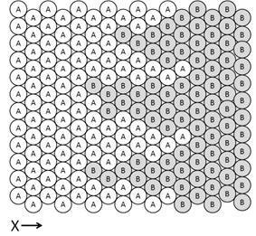
That the logistic function might provide a reasonable representation of an interface is suggested by the following argument. If we represent an interface between spheres labeled A and B as in the cartoon to the left, the probability that an exchange of two neighboring spheres in a horizontal direction will result in the interchange of an A sphere and a B sphere is PAB = k fAfB' =k fA(1 -fA')where fA is the fraction of A in a particular layer at X, fA' and fB' are the fractions of A and B in the neighboring layer X + dX, and k is some measure of the propensity for exchange. This, plus the fact that at some distance from the interface the material is either pure A or pure B, suggests that the change in fA as a function of X can be expressed as dfA/dX= kfA(1–fA), which, upon integration, gives fA= 1 / (1 + e-kX). Since k will have the units of 1/X, we can replace k by 1/D where D has the units of X. Furthermore, if Y is an instrument response to a measurement of species A so that Y is proportional to the fraction fA, then Y will be given by Y = A / (1 + e(X–Xo) / D) where X0 is the midpoint of the interface where Y = A / 2. Y varies from A to 0 through the interface. The parameter D is seen to be a scaling parameter that defines the width of the interface. As D?0, the profile of Y approaches a step function.
The scaling parameter itself may not be constant. If the spheres in the cartoon above were, for example, of a different size, the rate of change in fA with X might well vary with X. If we allow D to vary logistically with its own scaling factor, for example,
D = 2 D0/ (1 + e Q( X– Xo)),
the sigmoidal shape will be sharper at one side of the interface than the other.
If we now allow the pre and post interface baselines to be non-zero and furthermore allow for instrument response drift in the form of a quadratic equation in X, the full extended logistic function becomes:
![]()
Depth profile measurements are complex processes (see, for example, S. Hofmann, Rep. Prog. Phys. 61 (1998) 827-888 and references quoted therein.) This empirical approach in no way should suggest that the extended logistic function is being advocated as an atomic scale model for describing depth profile analyses. It merely provides a convenient and reasonable means for estimating the position, width and asymmetry of the interfacial profile in a systematic fashion from a set of discrete measurements.
Credit: Image, NIST
Contact
-
(301) 975-3949