Modeling and analysis

Different approaches exist for estimating greenhouse gas emissions across a city or region, which are typically classified into top-down and bottom-up methods.  Top-down methods often incorporate atmospheric transport and dispersion modeling with inverse models to estimate fluxes. Bottom-up methods often use reported emissions, process-based models, and/or activity data to estimate fluxes either from anthropogenic activities or the biosphere.

Top-down methods

Atmospheric transport and dispersion modeling

Transport modeling is often used to interpret concentration measurements from the atmosphere.  In order to determine the location and magnitude of a GHG emissions source using an atmospheric measurement, we need to simulate the transport of the gas from its emissions source to the location of the measurement.  For the NEC project, we are using various meteorological simulations, including the Weather Research and Forecast (WRF) model, coupled with Lagrangian particle dispersion models (e.g. STILT or HYSPLIT) to accomplish this.  The transport model output is then used in atmospheric inverse models to estimate fluxes.

Inverse models

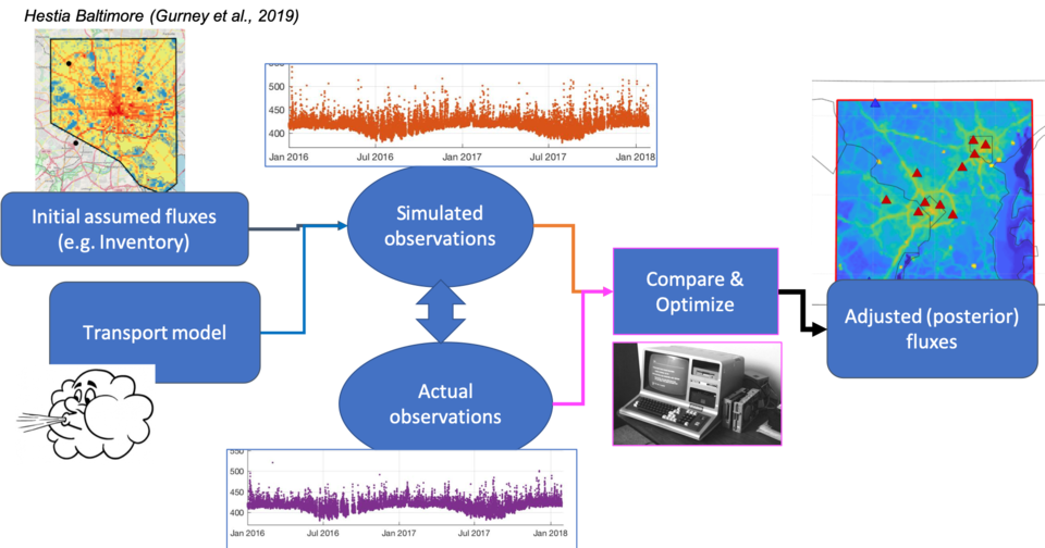
At their most basic, atmospheric inverse models rely on atmospheric measurements of greenhouse gases, and an atmospheric transport model to infer the most likely distribution of emissions, or GHG fluxes, at the earth surface upwind of the measurement locations.  Because they interpret the atmospheric footprint of all emission sources, inverse models can provide an independent constraint on bottom-up estimates of GHG flux.  In the most typical use of atmospheric inverse models, a Bayesian approach is applied, where bottom-up inventories are used as prior estimates, which are then updated using the atmospheric data constraint.  This data-fusion approach takes advantage of all possible information relating to GHG emission activity, although it can then be difficult to disentangle errors coming from the different data sources.  At NIST, we use different flavors of Bayesian inversion approaches, including the geostatistical method which relies on the atmospheric data constraint as much as possible to estimate fluxes and covariance parameters used in the inversions.  Geostatistical inversions are also used not just to estimate GHG fluxes, but also to evaluate the quality of different inventory products and biogenic flux models in terms of their ability to explain the observed emissions signal in the atmosphere.

NEC-BW and regional inversions

NIST researchers are currently working on developing atmospheric inversion models for the metropolitan area of Washington D.C. and Baltimore (NEC-BW) to estimate both CO₂ and CH₄ fluxes at a 1 km spatial resolution using an expanded measurement network in the region funded by NIST and maintained by Earth Networks.  In addition, these city-scale inversions can take advantage of data from dedicated flight campaigns measuring GHG concentrations upwind and downwind of the region. 

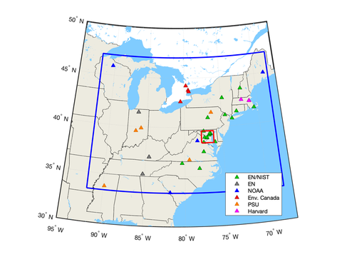
Urban inversions require the specification of GHG mole fractions in incoming air flowing into the region, the influence of which can be subtracted out of the observed mole fractions collected within the region.  Given that the NEC-BW is downwind of the entire North American continent with large emission sources, getting these background conditions right is critical for accurately determining net emissions within the domain of interest.  To help address this issue, NIST scientists are also developing a larger regional inversion for the eastern US and Canada at a coarser spatial scale (0.1 degrees), which can help to constrain these boundary conditions by explicitly solving for fluxes in areas upwind of the NEC-BW (Figure 3). 

Using the NEC-BW urban and regional inversions as a testbed, NIST scientists are working to quantify and reduce uncertainties from the inversion models: not just from the background conditions, but also uncertainties associated with the inversion setup, bottom-up flux estimates, transport model errors and noisy observational data.  An additional challenge remains to adequately identify the influence of anthropogenic emissions in the total GHG flux, given large contributions from biospheric activity, particularly for CO₂ during the growing season, but also for CH₄ near wetlands.  Towards this end, NIST researchers are working on generating and improving biospheric models that can help to separate the anthropogenic and biogenic flux contributions.  Ultimately, the goal of all this work, in collaboration with partners working in other urban testbeds, is to develop a set of best practices for urban inversions for GHG emission monitoring in the United States and beyond. 

Bottom-up methods

Gridded anthropogenic CO₂ emission inventories are developed by incorporating data on fuel sales, traffic counts, building operations, and power plant electricity generation, as well as point-source emissions from other industrial activities.  Different products exist for the coterminous U.S. (e.g. Vulcan) and for specific cities (e.g. Hestia) in Los Angeles, Baltimore, Indianapolis) at higher spatial and temporal resolutions.  Other global CO₂ emission inventory products (e.g. ODIAC, FFDAS) downscale emissions from national and regional totals to the grid-scale.  CH₄ emission inventories (e.g. EPA, EDGAR) also exist, but typically have higher uncertainties than for CO₂.  Different products can have higher quality for specific regions and spatiotemporal scales compared to other products and can thus be more suitable for specific applications.

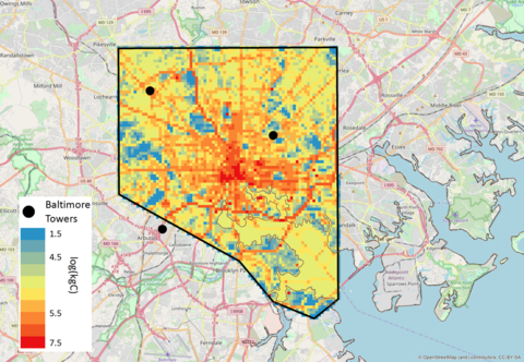
Hestia Urban Datasets are available for Los Angeles, Indianapolis, Baltimore, and Salt Lake City.